Active borehole: In the Borehole Manager, the check-boxes beside the borehole names are used to "enable" or "activate" the borehole. The data listed for active boreholes will be included in gridding and solid modeling processes; the data for inactive boreholes will not. Active boreholes will be displayed in section, profile, and fence diagram panel-picking windows; inactive boreholes will not.
ASCII: American Standard Code for Information Interchange file. ASCII files are also referred to as "text" files. RockWorks now expands upon this standard to support textual files which contain non-Latin characters ("unicode").
ATD Files: RockWorks2002 - RockWorks15 stored data in the RockWorks Datasheet in an ASCII (text) tab-delimited format, with the file name extension ".atd." These files contain a header block followed by rows and columns of data, with tab characters separating the columns. This file format has been replaced by ".rwDat". ATD files can be read in the current version of RockWorks and updated to the new format.
Borehole Manager: One of two main data windows in RockWorks, the Borehole Manager contains a database for entry of subsurface borehole data: well locations, stratigraphy, lithology, geochemistry / geophysical / geotechnical measurements, fractures, water levels, log symbols/patterns/well construction information for use in generating strip logs, cross sections, solid models, fence diagrams, and surface models. It supports vertical and deviated boreholes. Each borehole is stored as a record in a project database (by default SQLite format) in the current project folder. SQL Server databases are supported in the RockWorks Advanced level. The Borehole Manager contains its own set of program tools and menus at the top of the window. See also the RockWorks Utilities.
Central Meridian: In order to perform a coordinate conversion to UTM meters or feet from another coordinate system, the "central meridian" for the UTM "zone" must be selected. The Central Meridian you choose will determine the output longitude (Easting) coordinate range. Typically, the chosen Central Meridian should be as close to the center of the longitude coordinate range as possible. The accuracy of the translation is greatest within a single UTM zone and decreases the farther each zone is from the zone of the selected Central Meridian. The Central Meridians range from -177 western longitude (UTM Zone 1) to 177 eastern longitude (UTM Zone 60).
Color Model: RockWorks contains tools to interpolate a grid or solid model from downhole color measurements, XYZ points with colors, or even raster images displayed in 3D.
Like modeling other measured values (such as geochemistry), you can choose from a variety of modeling methods and options. * Unlike modeling other data types, the color modeling process will store an actual Windows color for the node. For example, a node value of 0 would represent black, 16512 would represent dark brown, 10864606 would represent light tan, 16777216 = white, and so on. For this reason, RockPlot2D and RockPlot3D offer a "direct" method of coloration, grabbing the node values directly for color assignments, rather than assigning a gradational color scheme to this type of data. Be sure the "Z = Color" or "G = Color" options are activated in the Gridding Options or Solid Modeling Options windows.
(* Don't use the "distance-to-point", "cumulative", or "sample-density" algorithms for gridding or 3D modeling of color data.)
Column Separator: See Delimiter
Command Script: This provides a means of running most of RockWorks' processes using a "script", without having to display the program's menus. This works really well if you wish to automate repetitive tasks, such as creating standard maps, logs, cross sections of a monitoring area on a monthly basis, or re-creating dozens of images for a project when the data has changed. Command scripts can be easily created from within RockWorks Playlist by selecting the File | Export to Command Script option. Command scripts are typically run by double-clicking on the file in the Project Manager, and it will be loaded into the player. Command scripts can also be run from a command line parameter. See Using RockWare Command Scripts for more information. Command scripts require RockWorks Advanced.
Data Dictionaries: These are a collection of XML files stored in a "system" folder inside each project folder. They define the RockWorks database structure for that project.
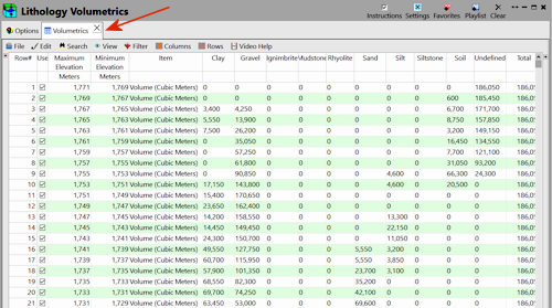
Data Tab: The row-and column results from many of the program computation tools (lithology and stratigraphy volumes, etc.) are displayed in a simple datasheet that is embedded in the options window. The results are accessible via the stick-up tab. You can use the File and Edit menu commands at the top of the window to transfer the data listing to the RockWorks Datasheet program tab (where more manipulation options are available), save the data to an external file, etc.
Datasheet: One of two main data windows in RockWorks, the Datasheet tab includes a datasheet for entry of non-borehole data: simple XYZ or XYZG, hydrochemistry data for Piper and Stiff plots, drawdown, survey mapping, lineation/planar data, to name just a few. The RockWorks Datasheet saves its row-and-column files in an "RwDat" file format (text). Datasheets can also bedisplayed as output inside the windows of programs which generate report output.
Decimals: When specifying decimal places consider the accuracy of your original data. For example, if you're recording lithology depths based on drill cuttings and counting rods, even one decimal place is not justified by the measurement technique. On the other hand, decimal degrees for longitude and latitude locations should be carried out to 6 decimal places.
![]()
To construct contours from your spreadsheet data, the Utilities | Maps | Triangulation Contours program does not construct a "grid model" as is done in the ModOps | Grid | Create menu programs. Instead, the Triangulation Contours program constructs a series of triangles with a data point at each vertex. The triangles are constructed so that the angles are as close as possible to equi-angular. (The program can display this triangle network as a map layer, see Network.) Contour lines are then interpolated between the triangle vertices and connected together to form the map. This process has been referred to as "dip-contouring" by some geologists.
Because it by-passes the gridding step, this mapping method operates the most quickly. In addition, it honors all of the data values; many people prefer this method of contouring since there is no loss of data integrity as a result of gridding.
This method can be used only for 2D maps since 3D surface mapping requires the generation of a data grid. Also, non-grid triangulation can leave blank areas in the map where there are no control points, unless you activate the "edge points." Contours tend to be very angular.
If Interpolate edge points is activated, this will force the program to insert points along the edge of the study area so that the contours can be drawn to the edge. It does this by inserting 5 points at equal spacing along the map boundaries (with one in each corner) and assigning them a value using the Inverse-Distance squared method. These new points can then be used when drawing the triangle network, assuring that all edges and corners are included within the network.
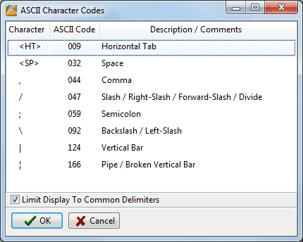
Delimiter: A "delimiter" is the character that separates columns within a text file. For example, some programs use the space character (#32) to separate data columns while others use tab (#9) characters. The following codes show some common delimiters:
Earth: A menu in the RockWorks Utilities program grouping, the Earth programs read spatial data from the RockWorks Datasheet for generation of diagrams for display in Google Earth: XY locations for display as icons or cones, image names for display as draped or as vertical panels, and much more.
In RockWorks16 the EarthApps had their own program tab and were available free of charge.
Easting: Eastings (also called the "X" coordinate) represent the east/west dimension within a Cartesian (xy) coordinate system. The RockWorks Utilities datasheet and the Borehole Manager database allow well or sample locations be defined in Eastings and Northings in feet or meters, in global or local units. It is assumed that Easting coordinates increase from west to east in your project.
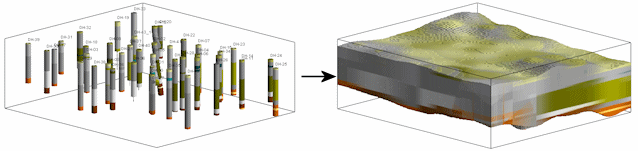
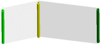
Fence Diagrams: Fence diagrams are one member of the family of 2D and 3D cross section diagrams available in RockWorks. Each behaves a little differently. Fence diagrams are available in the Lithology, Stratigraphy, I-Data, T-Data, P-Data, Fractures, Aquifers, and Colors menus.
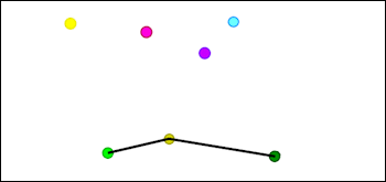
Fence diagrams represent one or more distinct slices through a 3D solid model, a 3D stratigraphic model or an aquifer model. A Fence diagram is created by selecting the beginning and ending points of each panel to be displayed in the 3D diagram. The panels can be placed anywhere within the model space. Striplogs can be displayed independently of the panels. (In the cartoon sequence below, the plan view of the borehole locations is rotated away from the viewer to achieve the 3D Fence Diagram view.)
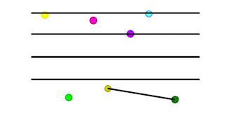
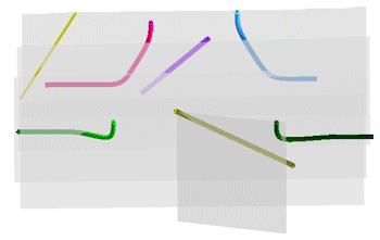
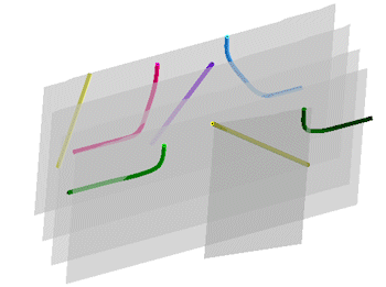
Because they are displayed in 3D, the orientation of the boreholes will be honored - vertical, inclined, and deviated borehole logs can be displayed in the 3D scene.
In RockWorks, drawing the fence panels is easily done on a plan-view display of the well locations (with optional raster background image), you can import the locations from an XY Pair table in the project database, or you can simply type in known coordinates for the Fence panel endpoints. Panels can be placed anywhere in the project space. The program will remember the location from one session to the next within the current project.
| Diagram type | No. Panels | Log orientation | Log Placement | 2D/3D |
| Section diagram | multiple | vertical only | at borehole locations | 2D |
| Profile diagram | 1 | true orientation | projected | 2D |
| Projected Section diagram | multiple | vertical only | projected | 2D |
| Fence diagram | multiple | true orientation | at borehole locations | 3D |
See Drawing Fence Diagram Panels for specifics.
Grid & Block Model Dimensions: The Grid & Block Model Dimensions (aka "Output Dimensions" or "Project Dimensions") are displayed in a pane at the top of the RockWorks program window, accessed via the Project Folder | Dimensions tab. They define for the program the spatial extents for all of your output grid models, solid models, 2D graphics, and 3D graphics. They also include the spacing of nodes along each of the three project axes, which will affect the density of grid models (X and Y) and solid models (X, Y, and Z).
The Grid & Block Model Dimensions represent the same coordinate system (UTM, State Plane, etc.) as your project data (which were defined when you created your project). While RockWorks permits your project data to contain mixed XY and Z (elevation, depth) units, the Grid & Block Model Dimensions must be one or the other - all feet or all meters - so that diagram scaling, volume computations, etc. are in the context of like units.
The Grid & Block Model Dimensions are important: The program will use them to know how big your project "space" is, and how large/small to scale your map and diagram components. (In RockWorks, map label sizes, log column widths, etc. are expressed as a percent of the size of the project.) The program will use them to know how big and how dense your surface models and solid models are supposed to be. It will use them as defaults for 2D and 3D axis labels. And more.
You can establish the Grid & Block Model Dimensions by typing them into the prompts, or you can use one of the Scan buttons to have the program scan your data to establish the dimensions. See Grid & Block Model Dimensions for more details.
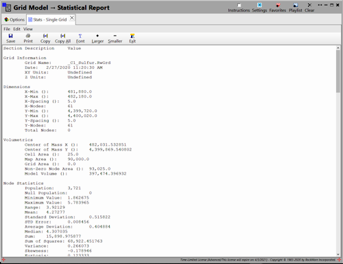
Grid Model: A grid model or grid file is the computer file of numbers that contains the results of the gridding process. It contains a listing of the X and Y location coordinates of the regularly-spaced grid nodes and the extrapolated Z value at each node. RockWorks grid models are stored in a mixed text/binary format. Grid models are stored in files with an ".RwGrd" file name extension.
A grid model is a numeric representation of a surface, be it elevations in your study area, formation thickness, or BTU values in a coal seam, to name a few.
Use the ModOps | Grid | Create | XYZ -> Grid program to create and display grid models from XYZ data for display as 2D or 3D images. Grid models are also created for drawdown surfaces (Hydro | Drawdown Surface), for lineation densities (ModOps | Grid | Create | Lineations -> Grid), and for volume computations (ModOps | Volume menu).
From the Borehole Manager, grid models are created when you create ground surface contours (Maps | Borehole Map), and display stratigraphic surfaces, isopachs, profiles, etc. (Stratigraphy menu) and water level surfaces (Aquifers menu). You can also extract grid models as slices from solid models.
Grid models can be summarized and manipulated in a variety of ways using the ModOps Grid menu tools. Use Grid | Filter to filter grid models, Grid | Edit to edit model nodes, Grid | Math to perform mathematical operations, and Grid | Import to import grid models from other sources . Statistical reports, node frequency diagrams, and observed v. computed XY plots are also available (Grid | Statistics).
You can also extract grid models from solid models (ModOps | Solid | Extract Grids menu).
Hang Section on Datum: This is an option in striplog sections (Striplogs | 2D Striplog Section) whereby the entire section is reset to an elevation of 0 at the top of a user-selected formation. This can be used to step back in time to the structure at that unit's deposition.
Important Notes:
WARNING: Logs and section panels can only be hung for boreholes that contain the selected unit. For your 2D sections, be sure to choose only boreholes that contain the selected formation. For 3D fences, it's probably best to turn off any boreholes that don't contain that formation. See Querying the Database for filtering tools.
Hole to Hole (Linear Interpolation) Stratigraphy Fence Diagram: These fences display stratigraphy correlation panels which are not created from interpolated surface models. Instead, the stratigraphic units are correlated with straight lines between like units in the boreholes on either end of the fence panel. These require that the fence panels are drawn between borehole locations. The panel endpoints will be snapped to coordinates of the closest borehole. These panels can honor inclined and deviated boreholes; for the latter the panels will attach to the logs at the panel tops and bottoms only.
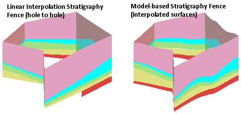
Comparison of fence diagram based on interpolated fence diagrams versus well-to-well fences:
| Linear Interpolation Fences | Model-Based Fences | |
| Method | Contacts based on linear correlations between adjacent boreholes. | Contacts based on interpolated surface models for all boreholes. |
| Appearance | Angular-looking correlations. | Smooth correlations. |
| Panel Locations | Panels must connect borehole locations. | Panels may be placed at arbitrary endpoints. |
See also: Interpolated Stratigraphy Fence Diagram
I-Data: This is the term we use to describe quantitative downhole data that was sampled at depth intervals. This might include geochemical measurements (concentrations, assays), percents (soil types), many geotechnical readings, etc. In earlier versions of RockWorks, this was referred to as "Geochemistry" data, but it certainly is not limited to that. I-Data is entered into the I-Data table in the Borehole Manager database, where you can define an unlimited number of columns for different sampled materials. I-Data can be represented on log diagrams as bargraphs (2D) or cylinders (3D). I-Data can be modeled into a 3D solid model using the I-Data menu tools and displayed graphically as a Profile (single slice), Section (multi-paneled profile), Fence (3D panels), 3D solid or isosurface diagram, and Plan map (horizontal slice). Levels are easily filtered and volumes displayed. You can use the View | Filter Boreholes and Select Boreholes tools to query based on I-Data values. I-Data entries are limited to numeric values only.
I-Text: This is the term we use to describe alphanumeric data that was sampled at depth intervals downhole. This might include comments, sample IDs, etc. I-Text is entered into the I-Text table in the Borehole Manager database, where you can define an unlimited number of columns for different sampled intervals. I-Text can be represented on log diagrams as text labels. I-Text entries can be alphabetic and/or numeric.
Installation Folder: RockWorks20x is a 64-bit application and the default installation location is C:\Program Files\RockWare\RockWorks20.
Isosurface: RockWorks offers display of solid model values as isosurfaces or using all voxels. What’s the difference? You might picture it like this:
In an isosurface diagram, the model’s G values are enclosed in a "skin" that is like a 3-dimensional contour. Within RockPlot3D you can interactively adjust the minimum value enclosed within the isosurface contour. For example, if you have a geochemistry solid model of lead values, and you wish to view the distribution of 5.23 ppb and above, you can set the isosurface contour level at "5.23" and see the skin surrounding voxels with G values 5.23 and greater. Such an isosurface is displayed in the image on the left.
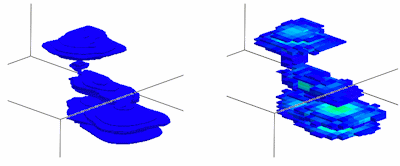
By contrast, in an all-voxel diagram, you’ll see color-coded voxels themselves, which usually look more angular and blocky than isosurfaces. In RockPlot3D you can filter out both high and low values from the display.
Generally, you should display lithology models using All Voxels. You'll usually display geochemistry and geophysical models using Isosurfaces.
KML Files, KMZ Files: These are "Keyhole Markup Language" files which are XML in format and which list spatially-referenced features for display in Google Earth. RockWorks generates the KMZ, or zipped, version via the Utilities | Earth programs, Animations | Google Earth programs, Images | Google Earth programs, RockPlot2D exports, RockPlot 3D exports, and other Google Earth output tools. RockWorks offers auto-launch of Google Earth, so that the contents of the KMZ file is loaded into the temporary places layer and displayed on the planet's surface.
LandBase: The RockWare Landbase is a database that you can download from the RockWare website, which contains Public Land Survey System (PLSS) data for a large portion of the United States. The LandBase can be used to generate lease maps and section maps for output to Google Earth or RockPlot2D. It can also be used to compute map locations (XY coordinates) for points or polygons which are described using only Range, Township, and Section descriptions. See RockWare Landbase Overview for details.
Latitude and Longitude: This is a global coordinate system that utilizes meridians (longitude) and parallels (latitude) to note specific points on the earth. Longitudes are measured east and west of the prime meridian which runs through Greenwich, England. There are 180 degrees of longitudes measuring eastward and westward; subdivisions are noted in minutes (60/degree) and seconds (60/min).
For mapping purposes, such as in the Utilities | Earth programs, RockWorks supports either decimal degrees (-105.209817) or annotated degrees (105°12'35.34"W) as input. For coordinate conversion purposes, such as in the Coords menu, you can also enter the coordinates in two separate columns (Degrees and decimal minutes, such as -105 | 12.589) or as three separate columns (Degrees, Minutes, and Seconds, as in -105 | 12 | 35.34). Eastern and Western longitudes are distinguished using the "East" or "West" notations or using a negative sign in front of Western coordinates; Northern and Southern latitudes use the "North" or "South" notations or use a negative sign in front of Southern coordinates.
If you are creating grid models and contour/point maps in the RockWorks ModOps or Utilities programs, the program will convert the coordinates to the project coordinates automatically; the resulting grid model and output map will represent the project coordinate system. There is also a coordinate converter which can convert lon/lat coordinates to another coordinate system, storing these in the current datasheet.
If you are working in the Borehole Manager and if you only have longitude and latitude coordinates for your well locations, you can enter those into the Other Coords tab (Borehole Manager Location table), using either decimal or annotated degrees, and then use the Edit | Coordinate Converter (to Easting/Northing) to convert these to the project coordinate system (in the Collar Coordinates tab).
Lithology Types Table: The Lithology Types Table is used to match lithology "keywords" in the Borehole Manager's Lithology data tables, such as "sand" or "limestone," to specific patterns and colors for representation in logs, profiles, fence diagrams, and block models. It is also used to define rock densities for mass computations, and "G" values for each rock type for solid modeling. A Lithology Types Table is stored in each project database.
You can view/edit the current project's Lithology Types Table by expanding the Project Tables/Types Tables heading in the Project Manager program tab, and double-clicking on the Lithology Types option. You can also access the Lithology Types Table via Borehole Manager "Lithology" data table, double-clicking in the "keyword" cell or by clicking on the Lithology Types button above the data listing.
LogPlot keywords, and lithology definitions from earlier versions of RockWorks are all fully importable.
MDB File: This is a Microsoft Access-compatible database file that was the default database format in RockWorks16 and earlier versions. This has been replaced by SQLite database (.sqlite File). You can request that RockWorks utilize an MDB database instead of SQLite by choosing the Customize Database Engine option when you create a new project. Earlier-version MDB databases can be updated automatically to the new .sqlite or .MDB database format using the Open Project menu option which walks you through the project-updating options.
Menu Settings: As you work in a project within RockWorks, most of the program settings are stored in two files on your computer. See RockWorks Menu Settings for additional details.
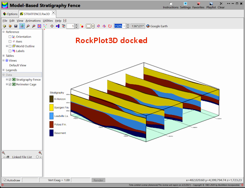
Model-Based Stratigraphy Fence Diagram: These fences display stratigraphy correlation panels which are created from stacked grid models of the different stratigraphic layers, displayed in 3D as if one or more slices were taken from anywhere in the project area. The slices or fence panels do not need to be aligned with borehole locations.
See above for comparison of these fence diagram types.
See also: Hole to Hole Stratigraphy Fence Diagram
Northing: Northings (also called the "Y" coordinate) represent the north/south dimension within a Cartesian (xy) coordinate system. The RockWorks datasheet and the Borehole Manager database allow well or sample locations be defined in Eastings and Northings in feet or meters, in global or local units. It is assumed that Northing coordinates increase from south to north in your project.
Null Value: This is a value you can use to "blank out" areas of a grid or solid model, so that they will not be displayed in a map or isosurface, or be included in area or volume calculations. In RockWorks, the null value is set to: -1.0e27 You can type this value into program prompts (such as the New Value prompt in the Grid Polygon filter) to assign the null value to applicable nodes. Many program menus also offer a Null radio button, and the value is assigned automatically.
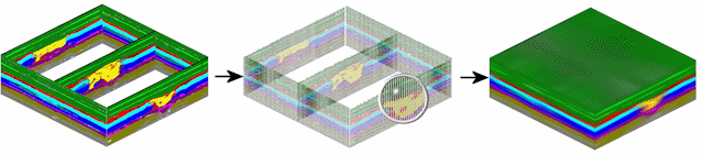
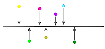
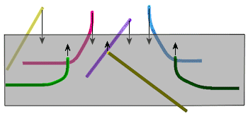
Onlap: The Onlap option, available in Stratigraphy Profile, Model-Based Section, Model-Based Projected Section, Model-Based Fence, and Layered Model programs, "fixes" models in which portions of an upper unit extend below the base of a lower unit. In order for this program to work correctly, the sequence of formations within the stratigraphy table must be listed from top to bottom (i.e. the younger formations at the top and the lower formations at the base.
In the non-onlapped model above left, the dark blue unit extends above the pink unit and above the base of the light blue. In addition, the green unit extends below the lower, yellow layer. Both result in "interference" patterns in the stratigraphic model. In the onlapped version, to the right, the light blue and pink units are set to to lie on top of the dark blue formation, and the green layer is set to lie on top of the yellow.
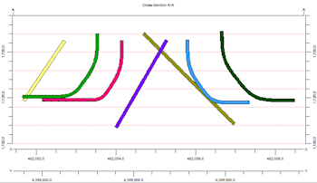
If you are dealing with non-sequential stratigraphic units, such as dikes, it is still possible to model the geology by disabling the Onlap feature and plotting the model as a voxels-only diagram:
P-Data: This is the term we use to describe quantitative downhole data that was sampled at depth points. This typically represents geophysical measurements (gamma, resistivity), but could also include point concentrations, etc. In earlier versions of RockWorks, this was referred to as "Geophysical" data, but it certainly is not limited to that. P-Data is entered into the P-Data table in the Borehole Manager database, where you can define an unlimited number of columns for different measurements. P-Data can be represented on log diagrams as curves (2D) or cylinders/oblates (3D). P-Data can be modeled into a 3D solid model using the P-Data menu tools and displayed graphically as a Profile (single slice), Section (multi-paneled profile), Projected Section, Fence (3D panels), 3D solid or isosurface diagram, and Plan map (horizontal slice). Levels are easily filtered and volumes displayed. You can use the View | Filter Boreholes and Select Boreholes tools to query based on P-Data values. P-Data entries are limited to numeric values only.
P-Text: This is the term we use to describe alphanumeric information that was collected at depth points downhole. This typically represents comments, sample IDs, etc. P-Text is entered into the P-Text table in the Borehole Manager, where you can define an unlimited number of columns for different measurements. P-Text can be represented on log diagrams as text labels. P-Text entries can be alphabetic and/or numeric.
Pattern Table: A Pattern Table is a RockWorks library of pattern designs, the dots, lines, and fills that repeat to make up rock type patterns. To load a different Pattern Table, expand the System Tables heading at the bottom of the Project Manager program tab, right-click on the "Patterns" item, select Set Pattern Location and browse for the RwPat file to be used. To view the pattern designs or to access the Pattern Editor, double-click on the "Patterns" item. The Pattern Table can also be accessed from the Lithology, Stratigraphy, Aquifer, and Well Construction Type Tables, and from the actual data tabs. RockWorks15 and LogPlot7 can share the same pattern library (.PAT files). Now RockWorks offers filled shapes in its patterns; its library is an .RwPat file.
Playlist: The Playlist tab in the main RockWorks program window is used to automate tasks that you do frequently in the program. Imagine that you are starting work in a new project and you create a borehole location map, a couple of striplog sections, and a T-Data Statistics map showing the high values of your contaminants. As new samples and monitoring wells are added, you can re-run these maps and diagrams with the click of a button, using all of the same settings. You can add items to a playlist with the click of a button in the program windows. The number of items you can store and run in a playlist is determined by the feature level of the program. See Using the RockWorks Playlist for details.
Principal Meridian: In the US Public Land Survey System, a Principal Meridian is a north-south line that divides Ranges into east and west. In a well location data file, you must list the Principal Meridian for each survey listing so that the program knows the "grouping" to which each Range and Township declaration belongs; this allows your data to span multiple meridians. However, when creating a Land Grid Section map, you may plot Range/Township/Section lines for only a single Principal Meridian at a time.
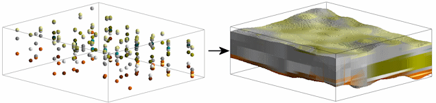
Profile Diagrams: Profile diagrams are one member of the family of 2D and 3D cross section diagrams available in RockWorks. Each behaves a little differently. Profile diagrams are available in the StripLogs, Lithology, Stratigraphy, I-Data, T-Data, P-Data, Fractures, Aquifers, and Colors menus.
Profile diagrams represent a single slice through your project. If you are displaying logs only (Striplogs menu) or if you are including logs with your modeled profile diagram, the logs are projected onto the single slice plane for those boreholes within a specified "swath" distance. (In the cartoon sequence below, the plan-view of the borehole locations is rotated away from the viewer to achieve the Profile Diagram.)
For single-slice Profile diagrams, the orientation of the logs will be honored - vertical, inclined, and deviated borehole logs will be displayed in the profile. In Profile diagrams, the distance between logs is determined by their perpendicular projection onto the profile line.
In RockWorks, drawing the profile line is easily done on a plan-view display of the well locations (with optional raster background image), you can import coordinates from a Profile Table in the project database, or you can simply type in known coordinates for the Profile endpoints. In addition, you can enter a filtering distance or "swath" to limit the projection of logs within this region. The Profile endpoints can be placed anywhere in the project area; they don't need to coincide with a borehole location. The program will remember the location from one session to the next within the current project.
| Diagram type | No. Panels | Log orientation | Profile type | Log Placement | 2/3D |
| Profile | 1 | true orientation | logs, models, models + logs | projected | 2D |
| Section | multiple | vertical only | logs, models, models + logs | at borehole locations | 2D |
| Projected Section | multiple | vertical only | logs, models, models + logs | projected | 2D |
| Fence | multiple | true orientation | models, models + logs | at borehole locations | 3D |
See Displaying Multiple Logs in a 2D Profile and Drawing a Profile Trace for specifics.
Project Folder: A Project Folder is a folder on your computer or network in which your RockWorks data will be stored. This includes the Rockworks database where the borehole data is stored, as well as datasheet files, program-interpolated grid and solid model files, output graphic files, playlist files, and command script files.
You can access a different project folder within RockWorks by clicking on the current project folder path that is displayed near the top of the program window, or by choosing the Project Folder | Open menu option. If you would like to be prompted for the Project Folder to work in each time the program launches, you can activate this setting in the Settings | Preferences menu.
In the Borehole Manager portion of the program, all of the borehole data is stored in a database file (.sqlite) that is automatically created when you create a new project folder, and assigned the same name as the project folder. The database also stores the project dimensions, as well as the lithology, stratigraphy, aquifer, and well construction reference tables associated with the project, and other project lookup tables. Along with the database, any grid models, solid models, fence panels, and graphics files will be stored in the current project folder.
Many of the programs in the RockWorks menu ribbon read data from the datasheet which are stored as .RwDAT files in the current project folder. Grid and solid models, and graphics files will also be stored in the project folder. You can use the same Project Folder for work in all of the RockWorks interfaces.
The contents of the current Project Folder will be displayed in the Project Manager program tab.
The database's data dictionaries are stored in a "system" folder inside each project folder, defining the database structure for that project.
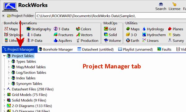
Project Manager: Is a main program tab which displays the files within the current project folder. It provides a means of viewing the files in the current project folder, opening files, previewing files, and more. You can dock the Project Manger alongside the Borehole Manager and Datasheet, if you prefer to have it handy while you are working in those program tabs.
Projected Section Diagrams: Projected section diagrams are one member of the family of 2D and 3D cross section diagrams available in RockWorks. Each behaves a little differently. Projected Section diagrams are available in the StripLogs, Lithology, Stratigraphy, I-Data, T-Data, P-Data, Fractures, Aquifers, and Colors menus.
Projected section diagrams represent multiple, connected slices through your project. If you are displaying logs only (StripLogs menu) or if you are including logs with your modeled Projected Section diagram, the logs are projected onto the multiple slice planes for those boreholes within a specified "swath" distance. (In the cartoon sequence below, the plan-view of the borehole locations is rotated away from the viewer and flattened to achieve the Projected Section Diagram.)
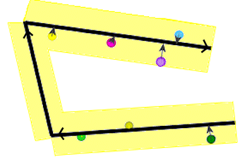
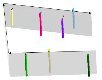
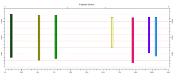
For multi-slice Projected Section diagrams, all boreholes are plotted as vertical. The distance between logs is determined by their perpendicular projection onto the projected section line.
A Projected Section diagram is created by selecting the endpoints of the slices which are to be displayed from left to right in the output diagram, and onto which the boreholes are to be projected. Drawing the section lines is easily done on a plan-view display of the borehole locations (with optional raster background image), an XY Coordinate table in the project database, or you can simply type in known coordinates for the Section vertices. In addition, you can enter a filtering distance or "swath" to limit the projection of logs within this region. The Projected Section endpoints can be placed anywhere in the project area; they don't need to coincide with a borehole location. The program will remember the location from one session to the next within the current project.
| Diagram type | No. Panels | Log orientation | Profile type | Log Placement | 2/3D |
| Profile | 1 | true orientation | logs, models, models + logs | projected | 2D |
| Section | multiple | vertical only | logs, models, models + logs | at borehole locations | 2D |
| Projected Section | multiple | vertical only | logs, models, models + logs | projected | 2D |
| Fence | multiple | true orientation | models, models + logs | at borehole locations | 3D |
See Displaying Multiple Logs in a 2D Hole to Hole Section and Drawing a Projected Section Trace for specifics.
R3DXML Files: This is the XML-based file format for RockPlot3D scenes from RockWorks15. These are text/XML in format and contain links to solid models, bitmap images, etc. that may be displayed in the RockPlot3D view. The file name extension is R3DXML. This file name extension replaced the more generic XML extension so that it can be specific to RockPlot3D. This has in turn been replaced by the ".Rw3D" file format in the current version RockWorks.
Right-Hand Rule: Convention whereby the dip direction is always 90-degrees clockwise from the strike. In other words, if you're looking along the axis of a strike that is 45-degrees (N45E), the dip will be 135-degrees (S45E), NOT 315 degrees (N45W). In other words, the dip direction is always to the right of the strike.
RK6 Files: These are files created by the RockPlot2D plotting window in RockWorks2006 - RockWorks15. You can open these into RockPlot2D; you'll be prompted to save the file under a new "Rw2D" name, and to establish the diagram type and units.
RKW Files; These are files created by the RockPlot2D plotting window in RockWorks2006 and earlier. You can open these into RockPlot2D; you'll be prompted to save the file under a new "Rw2D" name, and to establish the diagram type and units.
RockPlot2D Tab: RockPlot2D is the plotting window for flat (2D) graphics, such as maps, cross sections, stereonet diagrams, and the like. Starting in RockWorks15, the RockPlot2D window is embedded in the options windows, as a stick-up tab. You can also undock the image into a stand-alone window.
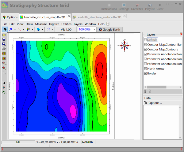
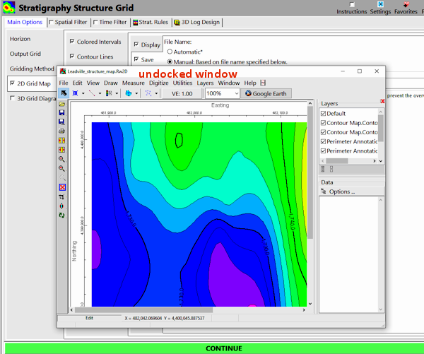
- Opening an existing file: Go to the Project Manager program tab, expand the 2D Diagrams heading, and double-click on the name of the Rw2D file you wish to view. It will open in a stand-alone window.
RockPlot3D Tab: RockPlot3D is the plotting window for three-dimensional graphics, such as solid model isosurfaces, fence diagrams, 3D surface images, 3D logs, and such. Starting in RockWorks15, the RockPlot3D window is embedded in the options windows as a stick-up tab. You can also undock the image into a stand-alone window.
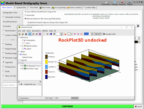
- Opening an existing file: Go to the Project Manager program tab in the main RockWorks window, expand the 3D Diagrams heading, and double-click on the name of the Rw3D file you wish to view. It will open in a stand-alone window.
RockWorks Menu Settings: Export the settings for the current program you're working in, by clicking on the Settings button at the top of the window and selecting Save Current Menu Settings to RwMnu File. These menu lists can be used to store a "snapshot" of the settings you are current working with. They can also be used by our support staff to trouble-shoot problems you're experiencing with the software. Use the Load Menu Settings from RwMnu File option to bring into the current menu an existing saved menu list. See RockWorks Menu Settings for more information.
Rw2D Files: These are files created by the RockPlot2D plotting window in RockWorks. These files store 2-dimensional (flat) images such as contour maps, ternary diagrams, 2D strip logs and cross sections, etc. When you choose Open or Save in RockPlot2D, you'll be opening or saving files in the Rw2D format. These are vector-based files, binary in format, and are specific to RockPlot2D. These files store your coordinate information, as well as the diagram type (map, chart, section). You can export from RockPlot2D to Google Earth, and to common image formats such as BMP, JPG, TIFF, DXF, and more. See Exporting RockPlot2D Files for information. If you try to open an "RK6" file created by RockPlot in an earlier version of RockWorks, the program will notify you that it will update the image to the newer graphic format, and allow you to assign a new file name, the diagram type, and coordinate information.
Rw3D Files: These are files created by the RockPlot3D plotting window in RockWorks. These XML-based files store 3-dimensional scenes such as 3D surfaces and logs, solid models, fence panels, etc. When you choose Open or Save in RockPlot3D, you'll be opening or saving files in the Rw3D format. These files store much of the data contained in a 3D scene, and they also contain links to external files such as bitmap images. Rw3D files store your coordinate information. You can export from RockPlot3D to Google Earth, and to common image formats such as BMP, JPG, PNG, and TIFF. See Exporting RockPlot3D Files for information. If you try to open an "R3DXML" file created by RockPlot in an earlier version of RockWorks, the program will notify you that it will update the scene to the newer graphic format, and allow you to assign a new file name and coordinate information.
RwDat Files: Data entered into the RockWorks Datasheet program tab are saved in files with the extension ".RwDat". These files contain a header block with geographic projection information, column titles, column types, data units, etc., followed by rows and columns of data. This format replaces older-version "ATD files." See Using the Datasheet for information.
RwDat Template Files: You can save the layout you've established for RwDat files (described above) for future datasheets. With the datasheet whose layout you wish to save displayed in the Datasheet program tab, choose File | Save As Template, and save this file with the default "rwdatTemplate" file name extension. Then, later, you can create a new datasheet with this same layout - column names, column types, metadata, etc. - using the File | New | Use Template menu option.
RwGrd Files: RockWorks grid models are saved in files with the extension ".RwGrd". These files contain a header block with coordinate information, followed by a binary block containing the model's node values. This format replaces older-version "GRD" files. See Gridding Reference for information.
RwMod Files: RockWorks solid models are saved in files with the extension ".RwMod". These files contain a header block with coordinate information, followed by a binary block containing the model node values. This format replaces older-version "MOD" files. See Solid Modeling Reference for information.
RWR Files: These are files created by the ReportWorks plotting window in RockWorks2006 and earlier. You can open these into newer versions of ReportWorks - the program will update them to the new RW6 format.
! However, if the old-format RWR files contain RockPlot RKW images from old versions of RockWorks, these images will not be updated. You'll need to update the RKW images to an Rw2D format (described above) and re-place them into the ReportWorks page.
RwRpt Files: These are files created by the ReportWorks page layout window. These files store page layouts, with inserted Rw2D images, bitmaps, text, and more. These are binary files, specific to the ReportWorks window. You can export from ReportWorks to common image formats, such as metafiles, bitmaps, and JPG images. See Exporting ReportWorks Files for information.
SDB File: This is a SQLite database file. SDB is the file name extension which was used in early releases of RockWorks17. It has been changed to .sqlite to provide more compatibility with third party programs, such as ArcGIS.
Section Diagrams: Section diagrams are one member of the family of 2D and 3D cross section diagrams available in RockWorks. Each behaves a little differently. Section diagrams are available in the StripLogs, Lithology, Stratigraphy, I-Data, T-Data, P-Data, Fractures, Aquifers, and Colors menus.
Section diagrams represent multiple slices through your project. A Section diagram is created by selecting individual boreholes, in any order, that are to be displayed from left to right in the diagram. Striplogs can be displayed at the panel junctions. (In the cartoon sequence below, the plan view of the borehole locations is rotated away from the viewer to achieve the Section Diagram view.)
For Section diagrams, all boreholes are plotted as vertical. The distance between logs is proportional to the physical distances between the boreholes on the ground. (There is an equal-spacing override in the Striplogs | 2D | Section diagrams.)
In RockWorks, drawing the section panels is easily done on a plan-view display of the well locations (with optional raster background image), you can import the locations from an XY Coordinate table in the project database, or you can simply type in known coordinates for the Section vertices. If you are creating a Striplog-only Section, or if you are including your logs with modeled Sections, the panel endpoints should lie at borehole locations. If you are creating a modeled Section with no borehole logs, the panels can be placed anywhere in the project space. The program will remember the location from one session to the next within the current project.
| Diagram type | No. Panels | Log orientation | Profile type | Log Placement | 2/3D |
| Profile | 1 | true orientation | logs, models, models + logs | projected | 2D |
| Section | multiple | vertical only | logs, models, models + logs | at borehole locations | 2D |
| Projected Section | multiple | vertical only | logs, models, models + logs | projected | 2D |
| Fence | multiple | true orientation | models, models + logs | at borehole locations | 3D |
See Displaying Multiple Logs in a 2D Hole to Hole Section and Drawing a Hole to Hole Section Trace for specifics.
Solid Model: A solid model is a 3-dimensional grid model, in which a solid modeling algorithm is used to extrapolate G values for fixed X (Easting), Y (Northing), and Z (elevation) coordinates. The G values can represent geochemical concentrations, geophysical measurements, lithology rock types, or any other spatially-related quantitative value. RockWorks solid models are stored in ".RwMod" files which are text and binary in format.
Use the ModOps | Solid | Create program to create a solid model of XYZG data listed in the RockWorks datasheet or an external text file. The Solid menu also contains a variety of solid model math, filtering, and editing tools.
If you have downhole data entered into the Borehole Manager, use the Lithology, I-Data, T-Data, P-Data, Vectors, Colors, or Fractures menu tools to create solid models of these data types. The models can be displayed as profiles, multi-panel profiles or "sections," fence diagrams, plan maps, 3D isosurface or all-voxel diagrams. You can also request that surface-based stratigraphic models be converted to a solid model (.RwMod) format for volume computations.
SQLite File: This is a SQLite database file that is the default database format in RockWorks. This replaces the Microsoft Access database (MDB File) used in RockWorks16 and earlier. MDB databases from RockWorks15 and RockWorks16 can be updated automatically to the new database format using the Open Project menu option; some Microsoft drivers are required.
Stratigraphy Types Table: The Stratigraphy Types Table is used to match formation names in the Borehole Manager's Stratigraphy datasheets, such as "Minnelusa Sandstone" or "Shale-1" to specific patterns and colors for representation in logs, surfaces, profiles, fence diagrams, and block models. It also defines stratigraphic order, from the ground downward - important for good modeling. The Table also contains other settings that control the pattern fill percent for the formations in strip logs, the "G" value for the formation for stratigraphic models, and the density converter should you wish to compute mass.
A Stratigraphy Types Table is created for each project database. You can view/edit the current Stratigraphy Types Table using the Project Manager program tab; expand the Project Tables/Types Tables heading and double-click on Stratigraphy Types. You can also access the Stratigraphy Types Table via Borehole Manager stratigraphy datasheets - just double-click in the "formation" cell or click on the Stratigraphy Types button above the data listing.
Symbol Table: A Symbol Table is a RockWorks library of symbol designs, the dots and lines that make up map symbols. To change the name of the Symbol Table that RockWorks is to use, expand the System Tables heading at the bottom of the Project Managerprogram tab, right-click on the Symbols item, choose Set Symbol Table location, and browse to the location of the ".SYM" library you wish to use. To view the symbol library or to access the Symbol Editor, double-click on the "Symbols" item. You can also access the Symbol Table from the Borehole Manager's Location datasheet (double-click on the displayed symbol) or from the RockWorks Datasheet (double-click on a symbol cell in a datasheet).
System Folder: RockWorks installs two System Folders for storage of global look-up tables and settings.
Text Tab: There are a number of programs in RockWorks that generate text reports. The text window can be embedded as a tab in the program window. You can undock the text window by clicking on the upper tab and dragging.
Unicode: This is a standard for text files which includes support for most of the world's alphabets, and which is also utilized by RockWorks. This is an expansion of the "ASCII" format which RockWorks previously relied on.
UTM Coordinates: Universal Transverse Mercator (UTM) coordinates are a global, Cartesian coordinate system that is N-S and E-W grid-based. In the UTM system, a network of zones is used to correct for errors when fitting the grid to the spherical Earth. These zones are defined by Central Meridians. As a result, the regions between the zones are located less accurately than the areas close to the meridians. Every USGS 7.5 minute topographical map depicts the UTM grid either as small, blue tick-marks along the borders, or as thin, black lines across the map. The UTM x-coordinates (called eastings) increase to the east, and the y-coordinates (northings) increase to the north. RockWorks contains tools to convert longitude and latitude coordinates to UTM, offering 23 coordinate projection schemes including NAD83 and NAD27.
Advantages of using a UTM coordinate system:
(1) The UTM distance units are consistent, unlike longitude and latitude coordinates in which a degree of latitude is not equal to a degree of longitude except on the equator.
(2) Coordinates are reported as either feet or meters.
(3) It's a true Cartesian system - no need to insert a minus sign before western or southern locations.
(4) The coordinate numbers, though they can be large, are easier to deal with than the degree/minute/second notations or 6-decimal-place notations of longitude and latitude coordinates.
Disadvantages:
(1) Some problems can arise when working in areas that overlap two zones.
(2) The grid is not exactly aligned along true north in many areas.
These disadvantages are insignificant, however, when compared with the simplicity and straightforward nature of the UTM system.
Vertical Exaggeration: The VE button at the top of the RockPlot2D display window ![]() can be used to define a specific vertical exaggeration for the current plot. This is typically used to make long, flat cross sections taller (VE > 1) or short, deep sections flatter (VE < 1).
can be used to define a specific vertical exaggeration for the current plot. This is typically used to make long, flat cross sections taller (VE > 1) or short, deep sections flatter (VE < 1).
You can pre-define the vertical stretch for section and profile diagrams by clicking on the Vertical Exaggeration tab in the program settings and defining the intended vertical exaggeration factor. Doing this tells the program in advance how much you want the diagram to be stretched, which allows RockWorks to generate better-looking axis annotation by compensating for this stretch.
Well Construction Types Table: The Well Construction Types Table is used to match material names in the Borehole Manager's Construction data table, such as "casing" or "screen" to specific patterns and colors for representation in log diagrams. A Well Construction Types Table is created for each project SQLite database. You can view/edit the Well Construction Types Table via the Project Manager program tab: expand the Project Tables/Types Tables heading and double-click on the Const Types item. You can also access it via the Well Construction data tables - just double-click in the "material" cell, or click on the Const Types button above the data listing.
World File: This is an ASCII (text) file used by GIS systems to locate raster map images. The World File describes the location, scale, and rotation of the image. Example/explanation of World File contents:
File Contents Explanation
1.2875536481 Line 1 = Width (in x-units) of each pixel.
0.0 Line 2 = Rotation about the y-axis.
0.0 Line 3 = Rotation about the x-axis.
-1.2738853503 Line 4 = Height (in y-units) of each pixel.
400.0000000000 Line 5 = X-coordinate at center of upper-leftmost pixel (northwest corner)
600.0000000000 Line 6 = Y-coordinate at center of upper-leftmost pixel (northeast corner).
X: See Easting.
XML Files: This is the file format for files created in the RockPlot3D window, to store the information in a 3-dimensional graphic image (3D surfaces and logs, solid models, fence panels, etc.). These are text in format and contain links to solid models, bitmap images, etc. that may be displayed in the RockPlot3D view. In current versions of RockWorks, the file name extension is "Rw3D". In earlier versions of RockWorks, the "R3DXML" and plain "XML" file name extensions were used.
Y: See Northing.
![]()