Create a Water Level Fence Diagram

RockWorks | Borehole Operations | Aquifers | Fence

Use this program to:

• Interpolate grid models for the upper and lower surfaces of a single aquifer or multiple aquifers listed for a particular date or date range in the Water Levels table, and
• Slice these grid models along multiple panels. Because surfaces are interpolated across the entire project, you can place the fence panels anywhere you like.

Numerous surface modeling options are offered. You may request regular fence panel spacing, in a variety of configurations, or you can draw your own panels. The completed fence diagram will be displayed in RockPlot3D. Multiple aquifers are supported.

Feature Level: RockWorks Standard and higher

Menu Options
Step-by-Step Summary
Tips

Menu Options

• Rules & Filters: Use the buttons at the top of the window to apply filters and rules for this program. (More info)
  • Spatial Filter: Filter the input data for the aquifer model based on XYZ location, filter the data to be displayed in striplogs, if activated. Note that these tools filter the data that is passed to the modeling and log-generating procedures.
  • Time Filter: Insert a check in this box at the top of the program window to filter the data based on date/time. If you have sampled aquifer levels on multiple dates, this is where you establish which dates are to be processed. Click this button to enter the filter settings. (More info)
    • Choose Exact to enter a specific date for the data is to be processed. The date you enter here should match the date you entered into the Water Levels data tables.
    • Click in the Range button if you want to process water level data for a range of dates, and then specify the starting and ending date and/or time for the data to be included in processing. (See Entering Water Level Data for details about how the dates are entered.)
      ! If you have multiple entries for a borehole for the selected date range, the program will include all of them when creating the model, in effect averaging them.
  • Stratigraphic Rules: Apply stratigraphy rules for stratigraphic logs, if activated.
  • 
    
• 3D Log Design
  Click here to choose which data items are to be displayed in the logs, if activated via the Striplogs checkbox below, and in which order. See Using the 3D Log Designer and the Visible Item Summary.
• 
  
• Fence Location
  Click on this button at the top of the window to draw, on a map display of your enabled boreholes, where the fence panels are to be placed. The most recent fence drawn for this project will be displayed (More info)
• 
  
• Location Map
  Insert a check in this tab, at the top of the window, to create, along with the fence diagram, a reference map that shows the fence panel locations.
  Click on this tab to set up the map options. (More info)

• 

  ---

• Aquifer(s) to Model
  Click this tab to select which aquifers are to be represented in the model.
  • All Aquifers: Choose this option if surfaces for all defined aquifers are to be created.
  • Single Aquifer: Choose this option if you wish to model a single aquifer only.
    • Aquifer: Click to the right to select the name of the aquifer you wish to model at this time. The names that are displayed are read from the current Aquifer Types Table. This table also defines the color to be used to represent the aquifer - it's the background color defined in the Pattern block.
    • 
      
• Modeling Options
  Click this tab to establish the gridding method, the grid dimensions, and other gridding options.
  • Dimensions: Use this tab to specify how the grid dimensions are to be established. Unless there's a specific reason to do otherwise, you should probably leave the grid dimensions set to the current project dimensions.
  • Algorithms: Select a gridding method for the interpolation of the surfaces.
  • Options: Establish the other general gridding options (declustering, logarithmic, high fidelity, etc.).
  • 
    
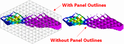
• Panel Borders
  Check this box to include a solid-line outline around each fence panel.
  Click on this tab to define the line style and color.

• 

  
  
• Surface Profile
  Insert a check here to include a solid line profile on each fence panel that represents a user-selected grid model, such as the ground surface.
  Click on this tab to select the grid model to be represented in the fence diagram, and to establish the profile settings. (More info)

• 

• Striplogs
  Check this item to include 3D logs with the aquifer fence display. Note that 3D logs for all active boreholes will be appended to the fence diagram.
  Click the 3D Log Design button at the top of the window to set up how you want the logs to look.
  Click on this tab to establish some additional striplog settings.
  • Clipping Dimensions: Insert a check in the X, Y, and/or Z axis options if you want to restrict the logs to a particular spatial area. (More info)
  • 
    
• Other 3D Diagram Options: Use these checkboxes to append other layers to your 3D scene. (Summary)
  
  • Draped Image: Include an image in this 3D scene, draped over an existing grid surface. (More info)
  • Floating Image: Include an image in this 3D scene, floating at a specified elevation. (More info)
  • Perimeter Cage Include a 3D reference cage around the fence diagram. (More info)
  • Legends: Include one or more legends with the diagram.(More info)
  • Infrastructure: Display buildings, pipes, or other infrastructure with your 3D scene. (More info)
  • Faults: Include 3D fault ribbons with this scene. (More info)
  • Other 3D Files: Include other, existing, RockPlot3D ".Rw3D" files in this scene. (More info)
  • 
    
• Output Options: Use these settings to define whether the output scene is to be displayed after it is created and how/whether it is to be saved in the project folder. (More info)
• 
  

Step-by-Step Summary

Follow these steps to create a 3D fence diagram illustrating the aquifer top and base on a user-selected date:

1. Access the Borehole Manager program tab.
2. Enter/import your data into the Borehole Manager, if you have not done so already. This program specifically reads location, orientation (if any), and water level data.
3. Enable boreholes: Be sure that all boreholes whose data are to be included in the aquifer model (which will be sliced for the fence diagram) are enabled.
4. Select the Borehole Operations | Aquifers | Fence command.
5. Enter the requested program settings, discussed above.
6. If you are including logs, be sure to click on the 3D Log Design tab at the top of the window to establish how you want the logs to look.
7. Click on the Fence Location tab at the top of the window to select the fence panel locations.
8. Click on the Continue button to proceed.

   The program will use the selected gridding algorithm to create grid models of the surface, base, and thickness of the selected aquifer, storing the models on disk ("date_top.RwGrd", "date_base.RwGrd" and "date_isopach.RwGrd"). The date portion of the file name should comply with the mm_dd_yyyy or dd_mm_yyyy date format as established in Windows.

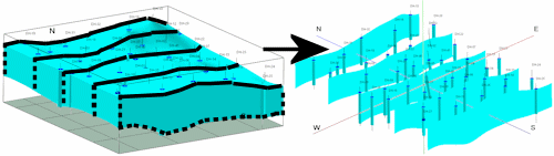
   RockWorks will then look at the coordinates specified for each fence panel and determine the closest nodes along that cut in each grid model. It will construct a vertical profile to illustrate the aquifer top and base elevations, using the color you specified. This process will be repeated for each fence panel you drew. Any other requested layers (logs, cage, etc.) will be appended to the 3D diagram. The completed view will be displayed in a RockPlot3D tab in the Options window.

9. You can adjust any of the program settings in the main Options tab to the left and then click the Continue button again to regenerate the fence diagram.
10. View / save / manipulate / print / export the fence in the RockPlot3D window.
    

Tips

• Use the File | Append tool to append stratigraphic diagrams or other 3D scenes to this fence.

See also

• Adding this program to your Playlist
• Adding this program to your Favorites
• Save/load/view menu settings
• 
  

Back to Aquifers Menu Summary

RockWare home page