Gridding Options

Faulted
Decluster
Logarithmic
High Fidelity
Polyenhance
Densify
Distance
Polygon
Smoothing
Z=Color
Undefined

Faulted: Insert a check here to apply faulting to the gridded surface(s). In RockWorks, this faulting process creates a barrier between nodes and control points such that if a fault segment lies between the grid node being interpolated and the control point(s) to be used in assigning its value, the control points' distances will be multiplied by a multiplier of 10. The result is that the control points will exert virtually no influence on the grid node, thus creating the barrier effect.
The program will use the active faults which are defined in the Faults tab in the main program window. (More info)

! The names of the enabled faults will be stored in the grid model itself (see RockWorks grid file format).
! If you are creating a map with line or color contours, you can include a map layer illustrating the fault polylines.
! If you are creating 3D surfaces, you can include diagram layers showing the faults as polyline intersections with the surfaces and/or the 3D fault meshes.
Decluster: Insert a check here to activate Declustering, which will remove duplicate points and de-cluster clustered points. This essentially creates a temporary grid in which a rectangle enclosing the control points is recursively subdivided into quadrants that contain control points until they are smaller than the specified maximimum cell size (below). The program then looks for multiple occurances of control points within each of these cells and replaces these control points with a single point based on the user-specified declustering method. Any pre-grid cells with no data points are discarded. It is the pre-gridded data that is then sent on to the surface modeling routine. This method works nicely if you have data sampled along lines or in clusters, such as along seismic lines. It can be used with any of the gridding methods. There is typically no speed benefits when declustering points for gridding; instead, the advantages are geared toward minimizing the influence of clustered points and eliminating the duplicates.
- Declustering Method
  - Average: The average Z-value for all points within a voxel.
  - Closest Point: The Z-value for the point that is closest to the voxel midpoint.
  - Distance Weighted: The estimated Z-value based on an inverse-distance-squared weighting algorithm. Recommended for modeling most data sets.
  - Highest: The highest G-value for all points that reside within a voxel.
  - Lowest: The lowest G-Value for all points that reside within a voxel.
- Horizontal Resolution: This defines the declustering cell size as a function of the specified project dimensions. For example, if the Horizontal Resolution is set to 50% (the default) and the x-spacing for the project model is 100', the horizontal size of a declustering cell will be 50'.
- Show Report: Check this to have the program display a window that summarizes how many points were consolidated via the declustering process. In addition, you'll have the option to copy the declustered points to the RockWorks Utilities Datasheet.
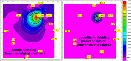
Logarithmic: The Logarithmic gridding option can be helpful for creating grid models of highly anomalous data. If activated, here’s how it works: The control point z-values are converted to natural logarithms. If a control point has a value less than or equal to zero, the logarithmic z-value will be set to zero. A grid model, based on the logarithmic data, is interpolated. The nodes within the grid model are then converted back to the original units by exponentiation. The control point z-values are converted back to their original units by exponentiation.
- Data sets that contain large "outliers" (i.e. values that are far beyond the typical range of data) are typically problematic when the goal is to highlight these anomalous regions. By computing and gridding the natural logarithm of the control point values, the regional effects of these outliers is more localized as shown by the following diagram. The net effect is to highlight anomalous regions (e.g. contaminant plumes).
- Note: The new logarithmic capability should be restricted to data sets that contain geochemical or geophysical data with grossly anomalous data points. It is not well suited for surface elevation data due to the fact that these data sets typically include negative z-values (i.e. sub-sea elevations).
High-Fidelity: When selected, this option will "tweak" the final grid model (after any smoothing has been applied) such that the contours will do a better job of honoring the control points, regardless of the algorithm or the grid smoothing (below). The capability uses a recursive algorithm that grids the residuals, adds them back into the original model, and repeats the process until the cumulative error drops below a threshold. Note that those cells that contain more than one control point are re-defined such that the node value equals the average of all of the control point values within the cell. The following example depicts some data (the "Davis" data set) that has been gridded (via Kriging), smoothed, and contoured (dashed blue lines). The red lines show the same grid with the "high-fidelity" option enabled. The green arrows show areas where the contours have been improved such that they honor the control points.
Polyenhance: Insert a check here to activate Polynomial Enhancement - a tool that works nicely if your data has any regional trend. If activated the program will fit a polynomial surface to your data and compute the residuals for each control point (representing the difference between the source z-value and the polynomial-computed z-value). The program will then grid the residuals using the selected gridding method (Triangulation, Inverse-Distance, etc.). The residuals grid and the polynomial grid are then added together.
- Automatic, 1st Order (etc.): If you turn on the polynomial enhancement, you may select Automatic to have the program compute the best-fitting polynomial for your data. Or, you can select the order of the polynomial yourself by clicking in one of the remaining radio buttons. See Trend Surface Gridding for more information about the polynomial orders. For a summary of how well each polynomial order fits your data, you can run, separately, a Trend Surface Report (ModOps | Grid | Statistics menu).
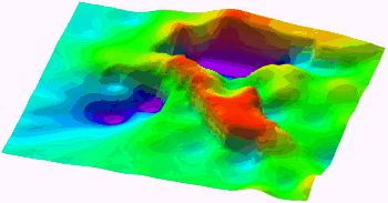
Densify: When activated, this feature will automatically add additional points to the xyz input by fitting a Delaunay triangulation network to the data and then adding the midpoint of each triangle to the list of xyz points.

The net result is that the subsequent gridding process is now using more control points which tends to constrain algorithms that may become "creative" in areas where there is little control.

Advantages: Reduces "bulls-eye" effect within inverse-distance-weighted modeling with small node spacings, restricts gridding to existing slopes, does not effect the fidelity of the gridding at the control points (unlike grid smoothing).
Disadvantages: Slows down the program, adding too many points (e.g. too many "passes") will eventually create a map/surface that is no different than a triangulation-based grid model.

Consider the following examples:
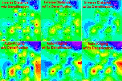
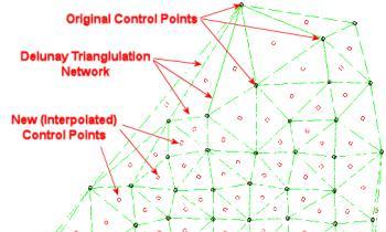
- Iterations: This represents the number of times the program will subdivide the triangles and thereby generate additional control points. The number of passes should typically not exceed one. Otherwise, the surface will begin to approximate a triangulated surface regardless of the gridding algorithm. Note that the program includes a special filter that will prevent the generation of numerous control points within areas of where the original control points are already close together.
- Save Points: Insert a check here to save a list of the original control points plus the added points in a text file.
  - Output File: Click here to type in a name for the text file to be created.
Distance: This option is used to define a value for grid nodes that are beyond a user-specified distance from a control point. The value that is assigned to these points may be either "null" (a special value that means "nothing" - as opposed to zero), or a user-specified value such as zero.
- Cutoff Distance (%): Enter here the distance beyond a control point, expressed as a percent of the project size, beyond which the grid nodes will be assigned a null or constant value.
- Replacement Value: Type in a specific value for the outlying nodes. If you want to use the RockWorks Null value (-1e27), click the Set to Null button.
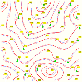
Here's a map illustrating a grid set to a maximum distance filter of 10% of the project area.
Polygon: Insert a check in the Polygon checkbox to activate a Polygon Filter. This filter will set the grid model’s nodes that lie either inside or outside of a polygon to a user-defined or null value. The polygon can come from a variety of sources.
- Filter Type: Select the operation:
  - Exterior: Choose this option to re-assign node values that lie outside the polygon to the replacement node value.
  - Interior: Choose this option to re-assign node values that lie inside the polygon to the replacement node value.
- Polygon Defined By:
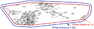
  - Automatic: Choose this option to request that the program define the polygon automatically, fitted around the periphery of the control points.
    - Offset Distance: Use this setting to expand the polygon outside the control points. Enter the map distance by which the polygon is to be enlarged.
  - Polygon Table: Choose this option if the polygon boundary is defined in a Polygon Table in the project database. Click to the right to choose the name of the polygon table to be used.
  - RwDat File: Choose this option if the polygon boundary coordinates are stored in an external RwDat file.
    - Polygon (RwDat) File: Click the Browse button to browse for the name of the RwDat file which contains the listing of vertex coordinates.
  - Rw2D File: Choose this option if the polygon(s) are defined in a RockPlot2D map.
    - Polygon (Rw2D) File: Click the Browse button to browse for the name of the Rw2D file which contains the map polygon(s).
- Replacement Value: Type in a specific value for the outlying nodes. If you want to use the RockWorks Null value (-1e27), click the Set to Null button.
Z = Color: Activate this option if the data you are gridding represents Windows color values. This tells the program to perform the requested gridding operations as normal, but to store the resulting data as an interpolated color value. Here is an example of how an X - Y - Color datasheet might look in the RockWorks Utilities.
! Note: Color-contouring a grid that has been generated with the "Z=Color" option turned on requires that the user set the color scheme to the "Direct (Node Value = Color)" setting.
Smoothing: Use this option to smooth the grid model to remove spurious "noise" and bring out broader trends. (This is also available as a filter within the Grid | Filters menu.)
- Method:
  - Distance Weighted Average: Choose this to smooth the grid node value using an averaging method that is weighted such that distant nodes will have less influence than closer nodes. This is the default method.
  - Lowest Z-Value: Using this method, the smoother will set the grid node to the lowest value within the search radius.
  - Highest Z-Value: Using this method, the smoother will set the grid node to the highest value within the search radius.
- Filter Size: This setting defines how many adjacent nodes should be used when smoothing each grid node. If you enter "1", then each node will be smoothed based on itself and the 8 nodes immediately surrounding it, 1 layer deep. If you enter "2", the node will be smoothed based on itself and the 24 nodes immediately surrounding it, 2 layers deep. The default settings is "1". The maximum setting is "100".
- Iterations: Enter the number of times the entire grid should be run through the smoother. The default setting is "1". The maximum setting is 100.
- Exclude Cells Based on Z-Value: Check this box to exclude grid nodes from the smoothing process based on their Z value.
  - Z-Min: Type in the minimum Z value to be omitted from smoothing.
  - Z-Max: Type in the maximum Z vlaue to be omitted from smoothing.
- Smooth Null Values: Check this option to include null nodes in the smoothing process.
  
  Note that the grid smoother will not smooth faulted regions if they are present in your grid model.
Undefined: Click on the Undefined tab to specify what value any undefined/filtered nodes are to be assigned. These are nodes which have been filtered based on polygons or distance, above.
- Set Undefined/Filtered Nodes to "Null": Click in this radio button to assign a RockWare null value (-1e27) to the replaced nodes. A "null" setting will set the filtered nodes to a value that RockWorks interprets as "undefined" thereby rendering these regions invisible when displaying the models. Null values are also excluded from area/volume calculations.
- Set Undefined/Filtered Nodes to...: Choose this option if you want to enter a specific value for the undefined or filtered nodes, and type that node into the prompt.

RockWare home page