Resampling Solid Models

RockWorks | ModOps | Solid | Math | Resample

This program reads an existing solid model and create a new model based on the current project dimensions. You can use this tool to resize solid models that are to be filtered against or run through mathematical operations with each other. Three methods are offered: sector-based averaging (slow), filter-based averaging (fast), and closest point (for lithology and stratigraphy models).

Feature Level: RockWorks Basic and higher

Menu Options
Step-by-Step Summary

Menu Options

• Rules & Filters: Use the buttons at the top of the window to apply filters and rules for this program. (More info)
  • Spatial Filter: Filter the input data to be displayed in striplogs, if activated.
  • Time Filter: Filter any T-Data or Aquifer data in striplogs, if activated.
  • Stratigraphic Rules: Apply stratigraphy rules for Stratigraphy data in striplogs, if activated.
• 3D Log Design
  If you decide to include logs with this diagram ("Striplogs" setting, below), click on this button at the top of the window to set up how you want the 3D logs to look.
  See Visible Item Summary and Using the 3D Log Designer for details.
• 
  

  ---

• Data Columns: Use these prompts to define the columns in the RockWorks Datasheet that list the XYZ(G) data from which the solid model was interpolated.
  ! These input prompts will be used ONLY IF you activate the Points layer in the diagram settings (see below). These settings will be ignored if you do not turn on the Points layer.
  • X (Easting), Y (Northing), Z (Elevation): Choose the datasheet columns where these input data are stored. These define the 3D location of the sample points.
  • 
    
• Input/Output Models
  • Input Model: Click to the right to browse for the name of the existing RockWorks solid model file (.RwMod) that the program is to read and manipulate.
  • 
    
  • Output Model: Click here to type in the name to assign to the new solid model file that the program will create, which results from the resampling operation.
  • 
    
• New Model Dimensions: Click here if you need to view or edit the current output dimensions. The output model will be generated using the current output dimensions settings. (See Viewing and Setting Your Output Dimensions.)
• 
  
• Resampling Options
  • Set Nodes Outside of Input Bounds to Null: Insert a check in this box if any nodes outside the extents of the original model are to be set to null. In other words, if you are resampling the input .RwMod file to larger dimensions, those outer nodes will not be assigned an interpolated value.
  • 
    
  • Resampling Method:
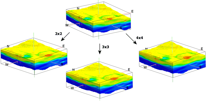
    • Filter Based (fast): Choose this option for a faster resampling method. Under this scheme, for each node in the output model, the program looks at the closest n nodes in the original model, and computes their average.
      2x2: average of the 4 closest nodes.
      3x3: average of the 9 closest nodes.
      4x4: average of the 16 closest nodes.
      The 2x2 filter is faster while the larger filters provide more smoothing. Filter-based resampling is significantly faster than sector-based resampling but may show some edge effects. The image below illustrates a solid model resampled to twice its density along all axes, using the different filters.

    • 

      
      
    • Sector Based (slow): Choose this option to use a sector-based resampling method. For each node within the new model, the program will locate the closest node from the original model within each quadrant. These nodes are then used to estimate (via an inverse-distance-squared algorithm) a value or the new node. WARNING: Unfortunately, this program is outrageously slow (assuming that the output model is larger than the input model) and should therefore be considered as a last resort when compared with re-modeling the original data.
    • Closest Point: Choose this option if you are resampling Lithology or Stratigraphy solid models, in which you don't want to get a gradational averaging of the node values. Instead, the value of the closest original node will be used for the resampled node, thus retaining the original material type classification.
    • 
      
• 3D Solid Diagram
  Insert a check here if you want to create a plottable 3D diagram of the resulting solid model.
  Click this tab to set up the diagram options.
  
  • Block Diagram
    • Isosurface: Click in the Isosurface radio button to display the solid model as if enclosed in a "skin." This view will be smoother than a voxel display. (More info)
      • Isomesh: Check this box to plot a series of polylines that represent three-dimensional contours at a user-defined cutoff. Click this tab to establish the settings. (More info)
    • Voxels: Click in the Voxels radio button to represent the solid model in the 3D display as color-coded voxels. You can choose to display either the Full Voxel, or just the Midpoint. Display of the midpoint only can significantly improve display time for huge models.
    • 
      
    • Filter: Check this option if you want to restrict the isosurface or voxel display to a specific data range. This does not affect the model, only the display of the model. Enabling this permits you to create an initial display in RockPlot3D that eliminates the need to manually change the display attributes. More importantly, this capability if essential for initially displaying the solid in a pre-filtered state when creating animations and Playlist scripts.
      ! These filter settings can be changed once the diagram is displayed in RockPlot3D.
    • 
      
    • Color Scheme: Choose the color scheme for the block model - automatic, table-based, etc. (More info)
    • 
      
  • Striplogs: Check this item to include 3D logs with the solid model display. Click the 3D Log Design button at the top of the window to set up how you want the logs to look.
    • XYZ Clipping: Check this sub-item if you want to restrict the logs to a particular spatial area. (More info)
    • 
      
  • Other 3D Solid Diagram Options: Use these checkboxes to append other layers to your 3D scene. (Summary)
    
    • Draped Image: Include an image in this 3D scene, draped over an existing grid surface. (More info)
    • Floating Image: Include an image in this 3D scene, floating at a specified elevation. (More info)
    • Perimeter Cage Include a 3D reference cage around the solid diagram. (More info)
    • Legends: Include one or more legends with the diagram.(More info)
    • Infrastructure: Display buildings, pipes, or other infrastructure with your 3D scene. (More info)
    • Faults: Include 3D fault ribbons with this scene. (More info)
    • Other 3D Files: Include other, existing, RockPlot3D ".Rw3D" files in this scene. (More info)
    • 
      
  • Output Options: Use these settings to define whether the output scene is to be saved (or displayed as "untitled"), how the file should be named, and whether it is to be displayed after it is created. It also offers export options. (More info)
  • 
    

Step-by-Step Summary

1. Select the ModOps | Solid | Math | Resample menu option.
2. Enter the requested menu settings, described above.
3. Click the Continue button to proceed.

   The program will load the input solid model file, recreate the new solid model using the new project dimensions and the selected method, and store the resulting solid model file on disk under the output file name you selected. If you have requested a diagram, it will be displayed in a RockPlot3D tab in the current window.

4. View / save / manipulate / print / export the diagram in the RockPlot3D window.
   

See also

• Adding this program to your Playlist
• Adding this program to your Favorites
• Save/load/view menu settings
• 
  

Back to Solid Menu Summary

RockWare home page