Create Detailed I-Data Volume Reports and Diagrams

RockWorks | Borehole Operations | I-Data | Volumetrics

This program is designed to perform a variety of "what-if" filtering operations and volume computing operations on an existing geochemical solid model. The input model can represent precious metal assays, contaminant concentrations, porosity values, or any measurable component for which you wish to compute volume. Throughout this section, we will refer to the modeled component generically as "material." 

This volume calculator specializes in models that are not stratified or homogeneous. You can filter the solid model for interbed thickness, material zone thickness, polygon areas, and distance from a borehole.

When the computations are complete, you have the options of:

• Storing the final computations as a Boolean solid model file that represents the distribution of favorable materials and/or
• Storing the final computations as a 2D grid file that represents either total thickness or mass, and/or
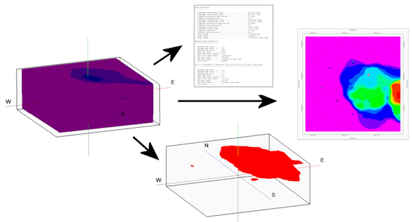
• Displaying the volume computations in a detailed or summarized text report, and/or
• Displaying the final solid Boolean model as a 3D diagram, and/or
• Displaying the final thickness or mass grid model as a 2-dimensional line or color-filled contour map or labeled cell map.

See also
     RockPlot3D for display of solid model or stratigraphy volume right in the 3D window.
     The Solid | Statistics | Report program for a quick report of dimensions and volume of any solid model.

Feature Level: RockWorks Standard and higher

Menu Options
Step-by-Step Summary

Menu Options

• Rules & Filters: Use the buttons at the top of the window to apply filters and rules for this program. (More info)
  • Spatial Filter: Filter the input data for the source data to be evaluated and for any 2D map layers that you include.
  • Time Filter: Filter any T-Data or Aquifer data in borehole maps, if activated.
  • Stratigraphic Rules: Apply stratigraphy rules for Stratigraphy data in striplogs, if activated.
  • 
    
• 3D Log Design
  If you decide to include logs with your voxel or isosurface diagram ("Striplogs" setting, below), click on this button at the top of the window to set up how you want the 3D logs to look.
  
  • Visible Items: Use the check-boxes in the first pane to select which log items are to be displayed. See Visible Item Summary for information about the different log items.
  • Options: Click on any of the Visible Items names to see the item's settings in the Options pane to the right. See the Visible Item Summary for links to the Options settings.
  • Layout Preview: For each item you've activated, you'll see a preview cartoon in the upper pane. Click and drag any item to the left or right to rearrange the log columns. See Using the 3D Log Designer.
  • 
    

• ---

• Track
  Click here to select the column in the I-data table that is represented in the solid model to be evaluated, below. The program will use this information when computing the distances between the control points and the solid model nodes.
  • Filter Based on G-Values: Activate this option to establish a data filter based on the measured values in the selected track. (More info.)
  • Resample at Regularly-Spaced Intervals: Check this box to resample the data. (More.)
  • 
    
• Input/Output Models
  Click here to define the models to be processed and the new models to be created.
  • Input
    • Ore Grade / Contaminant Solid Model (.RwMod): Click to to browse for the existing solid model to be read and processed for the volume computation.
    • Ground Surface Grid Model (.RwGrd): Click to browse for an existing grid model that represents the ground surface. Be sure this grid model has the same extents (X and Y min and max) and XY node spacing as the solid model above. This model will be used to identify above-ground nodes.
    • 
      
  • Output
    • Boolean Solid Model (.RwMod): Enter the name to assign to the final solid model that will contain the results of the volume filters, such as "PCB_volume.mod". This is a Boolean or "yes/no" model that contains node values of only 0 and 1; 0’s for areas where material is not present and 1’s where material is present.
      ! Don’t use the same name as the input solid model, above.
    • Thickness Grid Model (.RwGrd): Enter the name to be assigned to the 2-dimensional grid file that the program will create, containing the final thickness (or mass) values for material represented in the solid model, above.
    • 
      
• Acceptable Grade Range
  Use this to tell the program what range of data is to be included in the first Boolean solid model from which the reserves calculations are to be made. This grade (or "G") value range could represent favorable geochemistry (for example, G = gold assay values), unfavorable pollutant concentrations (G = parts per million), etc.
  • Minimum: Enter the minimum G value stored in the input solid model that is to be included in the volume computations. If you want all low values to be included, enter a large negative number, such as "-99999."
  • Maximum: Enter the maximum G value stored in the input solid model that is to be included in the volume computations. If you want all high values to be included, enter a large positive number such as "99999999."

  • At processing time, the program will use this information to create the initial Boolean (yes/no) solid model that will serve as the basis of the computations. Any voxels in the input solid model whose G values fall outside the indicated range will be assigned a 0 and any voxel nodes with G value inside the range will be assigned a 1.

    
    
• Interbed Filter
  Insert a check here if you want to remove small pockets of interbedded "waste" from surrounding "material" zones, translating them to "material" classification and including them in the reserves calculations. (Put another way, small pockets of Boolean model 0 values can be re-assigned a 1 for simplicity.) Example
  • Maximum Interbed Thickness: Type in the maximum thickness, in your depth or elevation units, to be considered as interbeds. Any contiguous "waste" voxels with a height less than this entry will be reassigned an "material" classification and set to a value of 1. How does it work?
  • 
    
• Thickness Filter, single zone
  Insert a check here to specify a minimum thickness for any individual material zone to be included in the reserves computations. This is a means of discarding non-economic areas from the totals.
  ! There is also a Total Thickness filter (next setting) that looks at multiple ore zones.
  • Minimum Acceptable Thickness: Enter the minimum thickness for a single, contiguous zone in a solid model column to be included in the volume calculations. How does it work?
  • 
    
• Total Thickness Filter, multiple zones
  Insert a check here to specify a minimum thickness for the combined, total material zones to be included in the reserves computations. This is a means of discarding non-economic areas from the totals.
  ! There is also a single zone thickness filter (previous topic) that filters individual material zones.
  • Minimum Total Ore Thickness: Here, type in the minimum combined thickness of all material zones found in each solid model column to be included in the volume calculations. How does it work?
  • 
    
• Stripping Ratio Filter
  Insert a check here to turn on and off a filter based on the ratio between the thickness of the overburden ("waste") and the thickness of the zone of interest ("material"). Several methods of computing the stripping ratio are offered, based on individual material zones or total material zones.
  • Maximum Stripping Ratio: Type the maximum acceptable value for the overburden:thickness ratio. Enter here just the real number overburden portion of the ratio (a ratio of 16:1 would be entered as "16"). The lower the stripping ratio, the thinner the overburden is in relation to the zone of interest. The higher the ratio, the thicker the overburden is in relation to the zone of interest. An example: A stripping ratio of 20:1 signifies that for every 1 foot of material thickness, 20 feet of overburden must be removed.
  • Method: Select how the program computes the stripping ratio. Choose one of the methods by clicking in its button.
    • Total Waste / Total Ore - The first option computes a single stripping ratio for each vertical column of nodes in the solid model, using total non-material thickness to total material thickness. If, for the column, the ratio exceeds your maximum, then all of the "material" for that column will be reclassified as "waste."
    • Contiguous Waste - The second option computes the ratio for each zone of material in each column of nodes in the solid model. For each zone it determines the total contiguous thickness of waste above it, up to the next material zone if any, and computes the stripping ratio for that zone. If, for that zone, the ratio exceeds your maximum, then that zone of material only is reclassified as "waste." 
    • Total Waste / Zones - The third option also computes the ratio for each zone of material in each column of nodes in the solid model. Unlike the previous method, this considers overburden for each material zone to be all of the overlying "waste" material, even the waste that lies above other material zones. If the stripping ratio exceeds your maximum, then that zone of material only is reclassified as "waste."  How does it work?
    • 
      
• Polygon Clipping Filter
  Insert a check here to turn on a spatial filter for the solid model. This spatial filter is based on a "polygon table," containing the X, Y coordinates for the perimeter of a polygonal area. All areas of your model that lie outside the polygon are excluded from the volume calculations.
  • Polygon Table: Click to the right to select the Polygon Table to be used.
    How does it work?
  • 
    
• Distance Filter
  This option is used to exclude from volume calculations those areas that exceed a user-declared distance from a control point (drill hole).
  • Maximum Distance: To the right, enter the distance measurement, in your X and Y and Z coordinate units, that you wish to declare as the maximum acceptable distance between a solid model voxel node and the nearest drill hole. Those nodes in your model that lie at a greater distance from a drill hole will not be included in the volume calculations.
    How does it work?
  • 
    
• Density Conversion (volume to mass)
  Insert a check here if you want the program to perform mass as well as volume computations. (See the important distinctions below.)
  • Density Conversion Factor: Click to the right to enter the value by which the volume units are to be multiplied to compute mass. The appropriate value to enter would depend on the density of the unit. Example: Let’s say your X, Y, and elevation units are in feet, so that the volume units will be in cubic feet. Then, let’s say you know your formation density is 0.014 tons per cubic foot. You would enter "0.014" in the Density Conversion Factor prompt.

    ! Be sure that the conversion factor you enter matches the volume units that the program is using! If the program will be computing volume in cubic feet but your conversion constant represents weight per cubic inch, you would need to convert the constant to weight per cubic foot before entering it here. These unit labels (such as "tons" in the above example) can be entered in the Create Report settings so that your units are correctly represented.

    ! This is Important: If you activate the Density Conversion utility, the following changes will be made to the program output:

    • The output report (if activated) will list computations in both volume units (such as "cubic feet") as well as mass units (such as "tons").
    • The output grid model will represent mass rather than thickness.
    • The output 2D or 3D surface map (if requested) will represent mass units (such as "tons") rather than thickness units (such as "feet").

    • See also: How to Measure Your Rock Density

• Create Report
  Check this item to request the creation of a textual report that lists all of the beginning, intermediate, and final program volume (and, optionally, mass) computations. If activated, the report will be loaded automatically into a text window upon completion.
  • Distance Qualifications: Insert a check in this box if you want the program to qualify the final computations as "proven," "probable," or "inferred" based on distances from drill holes. (Investors love this stuff.) Expand this to enter the distances in the prompts to the right.
    • "Proven" Cutoff Distance: Enter the node-to-drill hole distances, in your X Y Z coordinate units, that are to be categorized as Proven (high confidence).
    • "Probable" Cutoff Distance: Enter the node-to-drill hole distances, in your X Y Z coordinate units, that are to be categorized as Probable (medium confidence).
    • "Inferred" Cutoff Distance: Enter the node-to-drill hole distances, in your X Y Z coordinate units, that are to be categorized as Inferred or low confidence.

    • ! Lower categories are not inclusive of higher ones, so that Probable reserves do not include Proven reserves.
      How does it work?

  • Length Units: Type in the word(s) for the units in which the X, Y, and Z coordinates are reported in. The text you enter will be used in the output report. For example, if your X,Y,Z coordinates are in meters, you would enter "meters" at this prompt. Similarly, if X,Y, and Z are recorded in feet, you would enter "feet." 
  • Mass Units: Type in the words(s) for the units in which the mass computations, if activated, will be reported in, such as "tons." The unit name you enter here should match the Density Conversion conversion factor you entered.
  • Verbose: Insert a check in the Verbose check-box if you want the report to list complete summaries for all intermediate solid model files created during filtering. If this box is left un-checked, the report will list only final summaries of the models created during processing.
  • Decimal Places: In this prompt, enter the number of decimal places that are to be used in the reported values in the volume report.
  • 
    
• 2D Grid Map
  Insert a check in this check-box to request the plotting of the final thickness grid model (if no density conversion was requested) or mass grid model (if density conversion was requested) as a 2-dimensional map.
  Click this tab to set up the 2D map layers (bitmap, symbols, labels, line contours, color-filled contours, labeled cells, map border, etc.).
  • Output Options
    • Save Output File: Check this to assign a name for the map in advance, rather than displaying it as Untitled.
      • Automatic: Choose this option to have RockWorks assign the name automatically. It will use the name of the current program plus a numeric suffix, plus the ".Rw2D" file name extension.
      • Manual: Choose this option to type in a name of your own for this file.
    • Display Output: Check this option to have the resulting map displayed in RockPlot2D once it is created.
• • 
    
• 3D Solid Diagram
  Insert a check here if you want the final volume Boolean (material versus not-material) model displayed as a 3D voxel or isosurface diagram.
  Click this tab to set up the 3D solid layers (isosurface, voxels, reference cage, etc.).
  • Output Options
    
    • Save Output File: Check this to assign a name for the 3D scene in advance, rather than displaying it as Untitled.
      • Automatic: Choose this option to have RockWorks assign the name automatically. It will use the name of the current program plus a numeric suffix, plus the ".Rw3D" file name extension.
      • Manual: Choose this option to type in a name of your own for this RockPlot3D file.
    • Display Output: Check this option to have the resulting scene displayed in RockPlot3D once it is created.
    • 
      

Step-by-Step Summary

1. Open the project from which the input solid model was created.
2. Be sure you have an existing I-Data solid model (.RwMod) and a ground surface grid model (.RwGrd) for input.
3. Select the Borehole Operations | I-Data | Volumetrics menu option.
4. Enter the requested menu settings, described above.
5. Click the Continue button to proceed.

   The program will read the source solid model file and create a Boolean model of the requested G value range. It will then perform the requested filtering operations, storing the results of each pass in the Boolean model.

6. View the Report: If you have requested the creation of a volume report, the program will display it in a text tab in the Options window. At this time you can edit the report, save the report as a text file (Save button), or print the report (Print button).
7. View the Map: If you requested the plotting of a grid-based map to represent thickness values (or mass if the Density Conversion is activated) the program will display the completed image in a RockPlot2D tab.
8. View the 3D Surface: if you requested the plotting of the thickness or mass grid as a 3D surface, it will be displayed in a RockPlot3D tab.
9. View the Solid Diagram: If you requested the plotting of the final solid model, the program will display the completed image in a RockPlot3D tab.
10. You can adjust any of the volume or diagram settings in the main Options tab to the left and then click the Continue button again to recompute the volume statistics.
    

See also

• Adding this program to your Playlist
• Adding this program to your Favorites
• Save/load/view menu settings
• 
  

Back to I-Data Menu Summary

RockWare home page