RockWorks | ModOps | Volume | Ore Grid
This program is used to compute formation volume, given a column of thickness values in the datasheet, with a variety of filtering parameters. The computations are grid-based, with the gridding algorithm user-selected. Some of the advanced filtering operations include thickness, stripping ratio, up to 5 quantitative data column range restrictions, polygon areas, and distance.
The simple calculator offered in the Triangulation Volumetrics program computes thickness values using a Delaunay triangulation method. The grid-based reserves calculator uses a user-selected gridding technique which offers more flexibility.
What's most important is that this advanced method offers a variety of additional filtering "overlays" in which you declare desired values for associated spreadsheet columns, such as BTU measurements for a coal thickness model, or pollutant concentrations within a permeable zone. The program grids these variables (up to 5 of them) independently and then creates a "Yes/no" grid of each, in which nodes with values inside your desired range are set to "Yes" (or "1") and nodes with values outside the range are set to "no" (or "0").
The program internally multiplies the thickness model of interest by these Yes/no grids. Areas that correspond to any not-desirable areas of any of the Yes/no grids get set to zero and are not included in the final volume calculations.
In addition, you can invoke a polygon clipping filter so that only those thickness nodes within a user-entered polygon area are included in the computations. And, the output report can even list "Proven," "Probable," and "Inferred" reserves based on user-declaration of distance confidences.
This grid-based volume calculator offers several types of output:
- A grid file containing the numeric model for the final (filtered) grid of formation thickness values (or mass values, if requested), and
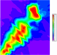
- A 2- or 3D map that illustrates the final thickness (or mass) grid, and/or
- A report that lists, in detail, the intermediate and final volume computations (with weight computations, if requested).
Feature Level: RockWorks Basic and higher
Menu Options
Step-by-Step Summary
- Data Columns
Click on this tab to define the input columns in the current datasheet for the volume calculations.
- X Column, Y Column: Use these drop-down boxes to select the names of the columns in the current datasheet that contain the X (Easting) and Y (Northing) location coordinates for the drill holes or sample sites.
Be sure you define your coordinate system and units.
- Thickness: Select the name of the data sheet column that contains the thickness values upon which the volume report will be based.
! RockWorks will convert the input units to the necessary output volume units.
- Overburden: Select the name of the datasheet column that contains thickness values of the overburden or layer that lies over the zone of interest.
- Output (Grid File): Click here to type in a name for the final, filtered thickness (or mass *) grid model that the program will create.
* If you have turned on the Density Conversion setting , the output grid file will represent mass units (volume X density conversion, such as "tons") rather than thickness units (such as "feet").
- Gridding Method
Click this tab to set up the gridding options.
- Dimensions: Click here to set the grid dimensions. Note that these gridding settings will apply to the original thickness grid model, as well as to any other filter models that are generated: stripping ratio, filters #1-#5, etc.
- Algorithm: Click this tab to select the gridding method and establish its settings, if necessary.
- Options: Establish the other general gridding options (smoothing, etc.).
- Generic Filters: These options are used to turn on and off volume filters based on additional data listed in your datasheet. These filters can be used to narrow the volumetric calculations based on additional measured parameters. You may turn on up to 5 additional filters, based on data read from data columns in the datasheet.
- Filter #1: Insert a check here to activate an additional data filter.
Example: Let's say that you are computing volume of a saturated zone, but only want those areas included where a pollutant concentration ranges from 0.5 to 1.4 parts per million. No problem! Just turn on Filter #1, specify the name of the column containing the pollutant's concentrations as the Data Column, and enter here the data range of 0.5 to 1.4.
- Minimum: Type in the minimum value in the data column selected for Filter #1 to be included in the computations.
- Maximum: Type in the maximum value in the data column selected for Filter #1 to be included in the computations.
- Filter Data Column: Select the name of the column in the datasheet where the filter data are listed.
- Filter #2: Insert a check here to activate a second additional data filter. Enter the Minimum and Maximum value to be included in the computations, and select the name of the datasheet column where these data are listed.
- Filter #3: Insert a check here to activate a third additional data filter. As mentioned above, enter the Minimum and Maximum value for this paramater to be included in the computations, and select the datasheet column where these values are listed.
- Filter #4: Check this box to activate a fourth additional data filter, enter the Minimum and Maximum values, and select the datasheet column where these data reside.
- Filter #5: Check this item to activate a fifth additional data filter, enter the Minimum and Maximum values, and select the datasheet column where these data reside.
- Thickness Filter: Insert a check here to apply a simple thickness filter. If this is activated, any values in the thickness model of your zone of interest that fall below the minimum thickness you enter will be set to zero and will be excluded from the computations. Type the minimum thickness value into the prompt.
- Stripping Ratio Filter: Insert a check here to apply a stripping ratio filter, which is based on the ratio between the thickness of the overburden and the thickness of the zone of interest. The overburden thickness is read from the data column you've specified for Overburden, above.
Type here the maximum acceptable value for the overburden:thickness ratio. Enter here just the real number overburden portion of the ratio (a ratio of 16:1 would be entered as "16").
The lower the stripping ratio, the thinner the overburden is in relation to the zone of interest. The higher the ratio, the thicker the overburden is in relation to the zone of interest. An example: A stripping ratio of 20:1 signifies that for every 1 foot of zone thickness, 20 feet of overburden must be removed.
- Polygon Clipping: Check this to turn on a spatial filter for the thickness grid. This spatial filter is based on a "polygon table," containing the X, Y coordinates for the perimeter of a polygonal area. All areas of your thickness grid that lie outside the polygon are excluded from the volume calculations.
- Polygon Table: Click here to select the name of the Polygon Table that you have created, containing the boundary coordinates of the polygon to be used to filter the input grid file. See Polygon Tables for information.
- Distance Filter: Insert a check in this box to exclude from volume calculations those areas that exceed a user-declared distance from a control point (drill hole) as defined by the X (Easting) and Y (Northing) locations in the datasheet.
Enter into the prompt the distance measurement, in your X and Y coordinate units, that you wish to declare as the maximum acceptable distance between a thickness grid node and the nearest control point. Those nodes in your thickness grid that lie at a greater distance from a control point will not be included in the volume calculations.
- Create Report: Activate this option to request the creation of a textual report that lists all of the beginning, intermediate, and final program volumetric (and, optionally, mass) computations.
- Classify: Check this option to apply proven, probable, and inferred classifications in the report.
- Distance Qualifications: Insert a check in this box if you want the program to qualify the final computations as "proven," "probable," or "inferred" based on distances from drill holes.

- Cutoff Distances: If activated, you will be requested to enter the node-to-control point distances, in your X and Y coordinate units, that are to be categorized as Proven (high confidence), Probable (medium confidence), or Inferred (low confidence). These will be isolated in the output report. Note that lower categories are not inclusive of higher ones, so that Probable reserves do NOT include Proven reserves.
- Volume-to-Mass:
- Density Conversion Factor: Enter the value by which the volume units are to be multiplied to compute mass. The appropriate value to enter would depend on the density of the unit.
- Example: Let's say your X, Y, and thickness units are in feet, so that the volume units will be in cubic feet. Then, let's say you know your formation density is 0.014 tons per cubic foot. You would enter "0.014" in the Density Conversion Factor prompt.
- Be sure that the conversion factor you enter matches the volume units that the program is using! If the program will be computing volume in cubic feet but your conversion constant represents weight per cubic inch, you would need to convert the constant to weight per cubic foot before entering it here. These unit labels (such as "tons" in the example below) can be entered in the Create Report settings so that your units are correctly represented.
- ! This is Important:
The Volume-to-Mass calculations mean the following:
* The output report (if activated) will list computations in both volume units (such as "cubic feet") as well as mass units (such as "tons").
* The output grid file (if saved) will contain node values representing mass units (such as "tons") rather than thickness units (such as "feet").
* The output map (if requested) will represent mass units (such as "tons") rather than thickness units (such as "feet").
- Labeling: Use this tab to define the words which will be used to label the calculations in the output report. Note that RockWorks will not check that you are entering the correct units.
- Item Being Evaluated: Enter the name of the item, such as "Ore", that you are working with.
- Area: Enter the label for area calculations in the report. For example, if your XY map coordinates represent feet, then the area would represent "Square Feet".
- G-Values: Enter the label for the quantitative values you're working with, such as "PPB".
- Length/distance: Enter the label for the length and distance measurements in the report. If your XY map units are in feet, then you would enter "feet" or "ft"; if they are in meters, you would enter "meters" or "m".
- Mass: Type in the label for the mass calculations, such as "tons". The correct label to use will be based on your volume units, and the Density Conversion Factor you entered above.
- Volume: Type in the label for the volume calculations, such as "cubic feet". The correct label to use will be based on your volume units.
- Decimals: For each item above, enter the number of decimal places that are to be used in the reported values in the volumetric report.
- Output Options
Click this tab to define the output format(s) for the report, whether the report is to be pre-assigned a name, and whether the report is to be displayed on completion. (More info)
- 2D Grid Map
Check this box to display the output grid as a 2D map at this time.
Click this tab to set up the 2D map layers (bitmap, symbols, labels, line contours, color-filled contours, labeled cells, map border, etc.).
- 3D Grid Diagram
Check this box to display the output grid as a 3D surface at this time.
Click this tab to set up the 3D map layers (surface colors, images, reference cage, etc.).
! You can request both a 2D and 3D representation of the grid model.
- Access the RockWorks Datasheet program tab.
- Open into the datasheet the file that contains (at minimum) columns containing X (Easting), Y (Northing), and thickness values. These coordinates and thickness measurements must represent the same units (e.g. all in feet or all in meters) so that the volumes make sense. Additional quantitative-data columns may be present, and can be used to constrain the volumes computed.
You might refer to the "Playlist_Coal_Data.RwDat" sample file for an example.
- Select the ModOps | Volume | Ore Grid menu option.
- Enter the requested input information, described above.
- Click Continue when you are ready to proceed.
- The program will perform the following operations.
- It will create a grid model of the zone of interest using the X, Y, and Thickness data specified in the Data Columns section of the window, using the gridding method, project dimensions, and other modeling options. This gives you the initial formation thickness model from which the volume can be computed.
- If you have activated Generic Filter #1:
- The program will create a grid model of the X, Y, Filter #1 data specified in the Input Columns section of the window.
- It will compare the value at each node in the Filter #1 grid to the value range you specified. All nodes that fall within the range are assigned a "1" and those that lie outside the range are assigned a "0". This Yes/no grid is stored temporarily.
- The thickness grid is multiplied by the acceptable Filter #1 Yes-no grid so that thickness values outside the desired value range are set to zero.
- The new thickness grid is stored in a temporary grid file.
- This process is repeated for Filter #2 through Filter #5, if they are activated.
- If you have activated the Thickness Filter:
- The program will compare each grid node value to the thickness filter minimum you specified.
- All nodes greater than or equal to the filter value are assigned a "1". All values that fall below the filter value are assigned a "0". This Yes-no grid is stored temporarily.
- The thickness grid is multiplied by the Yes-no grid so that thickness values below the minimum are set to zero.
- The new thickness grid is stored in a temporary grid file.
- If you have activated the Stripping Ratio Filter:
- The program will create a grid model of the overburden thickness using the X, Y, and Overburden data specified in the Data Columns section of the window, using the selected gridding method, project dimensions, and other modeling options.
- It divides each node's value in the overburden grid by the corresponding node value in the thickness grid, storing these overburden ratios in a temporary file.
- It compares each ratio grid node value to the stripping ratio maximum you entered.
- All nodes less than or equal to the filter value are assigned a "1". All values that are greater than the filter value are assigned a "0". This Yes-no grid is stored temporarily.
- The thickness grid is multiplied by the acceptable-overburden Yes-no grid so that thickness values greater than the maximum ratio are set to zero.
- The new thickness grid is stored in a temporary grid file.
- If you have activated the Polygon Clipping:
- RockWorks will determine which of the thickness grid model nodes lie within the polygonal area defined in the Polygon Vertex Table you've created. All nodes that lie on or within the polygon are assigned a value of "1". Those nodes that fall outside the polygon are assigned a value of "0". This Yes/no grid is stored temporarily.
- The thickness grid is multiplied by the polygon Yes/no grid so that thickness values outside the polygon are set to zero.
- The new thickness grid is stored in a temporary grid file.
- If you have activated the Distance Filter:
- The program will create a distance-to-point grid model of the study area, in which the node values represent the distance to the nearest drill hole.
- It will then determine which of the distance grid node values are less than or equal to your declared maximum distance. These are set to a value of "1". Those nodes with values greater than the declared maximum distance are assigned a value of "0". This Yes-no grid is stored temporarily.
- The thickness grid is multiplied by the distance Yes-no grid so that low-confidence nodes are set to zero and not included in the volume calculations.
- The new thickness grid is stored in a temporary grid file.
- If you have activated the Distance Qualifications option in the output report:
- RockWorks will create a distance-to-point grid model of the study area, in which the node values represent the distance to the nearest drill hole.
- The program then compares each distance measurement to the cutoff values you declared for each confidence interval.
- For each node in the Proven category, it stores the corresponding node value in the final, filtered thickness model in the first "group."
- For each node whose distance value falls in the Probable category, it stores the corresponding thickness value in the second "group."
- For nodes with distances in the Inferred category, corresponding thickness values are stored in a third group.
- Finally, those nodes with distances exceeding the furthest qualification are stored in a fourth group.
- The program then sums each group to determine total volumes in each of the qualification categories.
- If a mass conversion is requested, then the volume units are multiplied by the unit density to determine total mass.
If you have requested a volume report, the program will save it in the requested format(s) and display it as requested.
If you have requested a 2D map, it will be displayed in a RockPlot2D tab. Additional diagram-related items will appear within the main menu bar.
- If you have turned on the Density Conversion setting, the output map will represent mass units (volume X density conversion, such as "tons") rather than thickness units (such as "feet").
If you have requested a 3D surface, it will be displayed in a RockPlot3D tab. Additional diagram-related items will appear within the main menu bar.
- If you have turned on the Density Conversion setting, the output map will represent mass units (volume X density conversion, such as "tons") rather than thickness units (such as "feet").
- You can adjust any of the volume settings via the Options tab on the left and then click the Continue button again to recompute the volume and recreate the report/maps.
See RockPlot2D and/or RockPlot3D for complete documentation about manipulating the graphic images.
 Back to Volumetrics Menu Summary

RockWare home page