RockWorks | ModOps | Grid | Create | Single Elevation/Dip -> Grid
Use this program to create a new grid model that represents a flat plane with a user-defined elevation or a dipping plane based on a user defined orientation. If the plane is dipping, the user may define the xyz coordinates for a point that the dipping plane will intersect.
Feature Level: RockWorks Basic and higher
Menu Options
Step-by-Step Summary
- Rules & Filters
Use the tabs at the top of the window to apply spatial filters, time/date filters, or stratigraphic rules to data being displayed in your map layers. (More info)
- 3D Log Design
If you decide to include logs with this diagram ("Striplogs" setting, below), click on this button at the top of the window to set up how you want the 3D logs to look.
See Visible Item Summary and Using the 3D Log Designer for details.
- Grid to be Created: Click here to type in a name for the grid model (.RwGrd) which will be created.
- Dimensions: Click on this tab to view/adjust the grid dimensions.
- Orientation: The new grid model can be either a horizontal or inclined plane.
- Horizontal: Choose this option to set all nodes such that grid represents a horizontal plane.
- Elevation: Value to assign to all nodes within the grid model.
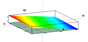
- Inclined: Choose this option to tilt the plane based on user-defined parameters.
- Dip Direction: Dip direction of the plane, in degrees. 0 = North. 90 = East. 180 = South. 270 = West.
- Reference Point: The output model will be adjusted such that the inclined plane intersects this point.
- X: Easting at reference point.
- Y: Northing at reference point.
- Z: Elevation at reference point.
- Dip Amount: Dip angle of the plane, in degrees. 0 = horizontal, -90 straight down. 90 = straight up.
- 2D Grid Map
Check this box to display the output grid as a 2D map at this time.
Click this tab to set up the 2D map layers (bitmap, symbols, labels, line contours, color-filled contours, labeled cells, map border, etc.).
- Output Options: Use these settings to define whether the output graphic is to be saved (or displayed as "untitled"), how the file should be named, and whether it is to be displayed after it is created. It also offers export options. (More info)
- 3D Grid Diagram
Check this box to display the output grid as a 3D surface at this time.
Click this tab to set up the 3D map layers (surface colors, images, reference cage, etc.).
! You can request both a 2D and 3D representation of the grid model.
- Output Options: Use these settings to define whether the output scene is to be saved (or displayed as "untitled"), how the file should be named, and whether it is to be displayed after it is created. It also offers export options. (More info)
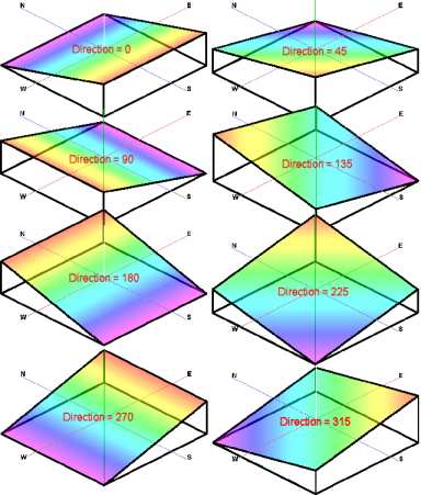
The following example depicts various dip directions with a constant dip angle of -15 degrees.
- Select the ModOps | Grid | Create | Single Elevation/Dip - Grid menu option.
- Enter the requested menu settings, as described above.
- Click the Continue button to proceed.
The program will generate a grid model with the dimensions you established. The Z values will be assigned either constant elevation values (flat) or those representing a tipped plane intersecting the defined reference point and the declared dip direction and angle. The resulting grid model will be stored under the file name you declared.
The requested diagram(s) will be displayed in a RockPlot2D tab and/or RockPlot3D tab in the Options window.
- You can adjust any of the settings via the Options tab to the left and then click the Continue button again to regenerate the diagram(s).
- View / save / manipulate / export / print the diagram in the RockPlot2D or RockPlot3D window.
Let's say that a strike and dip on the surface was measured for an important fracture orientation. The xyz coordinates for this point would be used as the reference point for an inclined plane. By plotting this plane in conjunction with other data (e.g. a stratigraphic block model), the viewer can see where the plane should intersect other features (assuming, of course, that fractures are perfect planes - which they aren't).
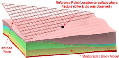
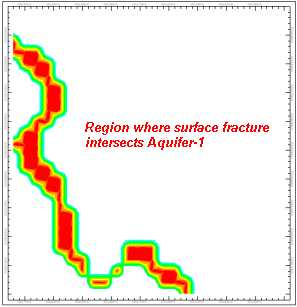
To isolate the exact intersection of two grid models, simply subtract one from the other (via the Grid-Math programs). Node values that approximate zero within the resultant grid model show where the surfaces intersect. In the following example, the fracture plane surface (as generated by this program) was subtracted from the Aquifer-1 (baby-blue in the diagram above) superface grid to create an intersection model. This grid was then converted to a Boolean grid as shown within the following grid.
 Back to Grid Menu Summary

RockWare home page