Creating a Gradient Vector Map

RockWorks | ModOps | Grid | Directional | Gradient Vector Map

This program reads a grid (surface) model and creates a 2D map containing small arrows at each grid node pointing either uphill or downhill. Arrows may be scaled and/or color-coded according to steepness of slope.

Note: This program requires that a RockWorks surface (grid) model already exist.

Menu Options
Step-by-Step Summary

Menu Options

• Input Grid
  • Grid Model Input File: Click to browse for the name of the existing grid model (".RwGrd" file) to be analyzed and displayed as a vector map.
  • 
    
• Vector Options
  • Direction: Choose the direction the gradient arrows are to represent, either Down-Gradient or Up-Gradient.
  • Length:
    • Choose Fixed if you want the map arrows to be the same length, roughly the same size as the node-to-node spacing.
    • Or, choose Proportional if you want each map arrow's length to be scaled based on its slope, with flat areas plotting with short arrows and steep arrows with long arrows.
  • Colors:
    • Choose Fixed to set the arrows to a single color, and click the color box to select the color.
    • Or, choose Proportional to set the arrows to a variable scheme, using cold colors for arrows between nodes with shallow slopes and hot colors for nodes with steep slopes, and graduating the colors in-between.
  • Frequency: Use this setting to define how many gradient arrows are to be generated in the map. A setting of "1" will include vectors for all nodes in the grid model. A setting of "2" will include vectors for every other node in the model. A setting of "3", every third node, and so on.
  • Filter: Enter the minimum and maximum slope values to be included in the map. Enter "0" for the minimum and "90" for the maximum if all nodes are to be included. Or, to show only those nodes with slope > 30 degrees, for example, you would enter "30" for the minimum and "90" for the maximum.
  • Thickness: Click here to select the line thickness for the arrows. "1" will generate thin lines, "3" thick ones.
    
    • Choose Fixed to set all of the arrows to a specific thickness. "1" will generate thin lines, "3" thick lines.
    • Choose Proportional to set the arrows to variable thickness, using thin lines to represent shallow slopes between nodes and thick lines for steep slopes between nodes, with intermediate thicknesses in between. You can choose the minimum and maximum thicknesses using the prompts.
  • Normalize Nodes: Leave this option unchecked if your grid model represents topographic elevations.
    If your grid model represents something other than topography (e.g. geochemical concentrations), you should check this box so that the Z values can be normalized to map units prior to computing the slope and aspect. For example, if a grid node spacing is 10 meters and the user is analyzing geochemical data than ranges between zero and 0.01, the maximum slope would be less than one degree in which case the program would produce a blank diagram. With normalization, however, the data is now rescaled to resemble a three-dimensional cube in which the slope will have a wide range (i.e. zero to 90 degrees).
    • Automatic: Using this normalization scheme, the program will rescale the grid node values such that the minimum node value will represent zero while the maximum node value will be equal to the map distance from the southwest corner to the northeast corner of the grid model. The map below illustrates a downgradient vector map based on normalized geochemical data that initially ranged between zero and 0.01.

    • 

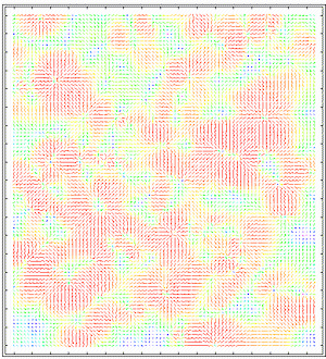
    • Manual: Choose this option if you want to enter your own min and max range within which the grid node values are to be normalized before the analysis is run.
    • 
      
• Background Image
  Check this option to display an image behind the other map layers. You can select your project image or another raster map.
  Click on this tab to establish the background-bitmap settings. (More info)
• 
  
• Labeled Axes
  Check this option to annotate the map borders with axis titles and/or coordinate labels.
  Click on this tab to establish the map axis settings. (More info).
• Map Overlays
  Check this option to include various other layers on your map. Options incude Infrastructure maps, US Public Land Grid maps, Polygon outlines, and more.
  Click on this tab to activate the different layers and establish their settings. (More info)
• 
  
• Other 2D Files
  Check this option to include existing RockWorks maps as layers with your map. For example, if you have a land grid map already created for your project, you can include that as a layer here.
  Click on this tab to select the existing maps (.Rw2D files) to be included. (More info)
• 
  
• Peripherals
  Check this option to include various map peripheral annotations with your map. Options include titles, north arrows, scalebars, and more.
  Click on this tab to activate the items and establish their settings. (More info)
• 
  
• Border
  Check this option to include a solid line border around the entire map image.
  Click on this tab to specify the line style, thickness, and color.
• 
  
• Output Options:
  • Save Output File: Check this to assign a name for the map in advance, rather than displaying it as Untitled.
    • Automatic: Choose this option to have RockWorks assign the name automatically. It will use the name of the current program plus a numeric suffix, plus the ".Rw2D" file name extension.
    • Manual: Choose this option to type in a name of your own for this file.
  • Display Output: Check this option to have the resulting map displayed in RockPlot2D once it is created.
  • 
    

Step-by-Step Summary

1. Be sure you have a RockWorks grid model (.RwGrd file) already created, for input into this program.
2. Select the ModOps | Grid | Directional | Grid | Gradient Vector Map menu option.
3. Enter the requested menu settings, described above.
4. Click the Process button to continue.

   The program will read the input grid model, compute slope and aspect for each node, and then create a map that indicates the up- or down-slope gradient (as requested) with arrows, using the requested map settings. The map will be displayed in a RockPlot2D tab in the Options window.

5. You can adjust any of the settings in the Options window (arrow settings, grid model name, etc.) and then click the Process button again to regenerate the map.
6. View / save / manipulate / export / print the map in the RockPlot2D window.
   

Tip: Use RockPlot2D's File | Export | RockPlot3D option to drape this downhill gradient map over the original grid surface for display in RockPlot3D.

See also

• Adding this program to your Playlist
• Adding this program to your Favorites
• Save/load/view menu settings
• 
  

Back to Grid Menu Summary

RockWare home page