Creating a Boolean Fault Model - Single Fault

RockWorks | Utilities | Faults | Single Dip List -> Boolean Fault Model

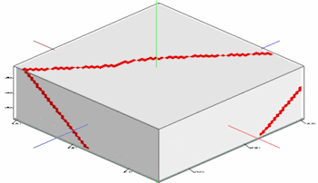
This program reads a list of dip data (e.g. points along a fault, contact, bedding plane) which includes XYZ coordinates, dip direction, and dip angle, and creates a 3D solid model (.RwMod file) in which the voxels intersected by the fault planes are assigned a value of "true" (1.0) and those which are not are assigned a value of "false" (0.0). This program offers a means of visualizing the 3D location of your faults.

! This program does not apply faulting to a solid model, it just shows the fault locations. While you can create the Boolean Fault Model in the Utilities interface, you need to have RockWorks Advanced to be able to use it to fault a 3D solid model.

See also: Plotting 3D Dip Ribbons - Single, Creating a 3D Fault File - Single Faults, Solid Model Faulting

Menu Options
Step-by-Step Summary

Menu Options

• Input Columns: The prompts along the left side of the window tell RockWorks which columns in the datasheet contain the input data.
  Click on an existing name to select a different name from the drop-down list. See a sample data layout below.
  • X: Column that contains the X or Easting coordinates for the fault polyline vertices.
    These can be Eastings in meters or feet, decimal longitudes, etc. See Defining your Datasheet Coordinates for more information.
  • Y: Column that contains the Y or Northing coordinates for the vertices.
    
  • Z: Column that contains the elevations where the measurements were taken. Be sure you've defined the elevation units in the column heading.
  • Dip Direction:  Choose the column that lists the direction, in degrees, toward which the fault plane is dipping.  (examples: North = 0, East = 90, South = 180, and West = 270.)
  • Dip Angle:  Choose the column that lists the dip angle.  Note: Horizontal is considered to be zero, and dipping straight down is entered as +90. 
    
    
• Direction Represents: Choose how the data listed in the data sheet are recorded.
  • Right Hand Rule: Using this convention, planar data are entered as strike bearing and dip angle, with the dip direction being 90 degrees clockwise from the strike azimuth bearing.
  • Dip Direction: Using this convention, planar data are entered with dip direction and dip angle.
    
    
• Declination Correction: Use this setting to correct for magnetic declination, in degrees.
  
  
• Distance Increment: This setting controls how finely the faulting panels will be subdivided, and is expressed as distance in your map units.
  
  
• Project Down-Dip: Insert a check to project the fault down-dip from the fault polyline.
  • Down-Dip Projection Distance: Click here to type in the distance, in your project units, for the projection. This is important - it will determine how deep the fault will extend in the model. If the fault planes are not consistent in depth, you'll need to break them up into separate files and create the Boolean Fault Model using multiple input files.

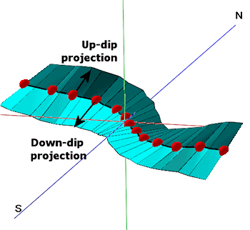
• Project Up-Dip: Insert a check here to project the fault up-dip from the fault polyline.
  • Up-Dip Projection Distance: Click here to type in the projection distance, in your project units.
    
    
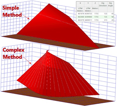
• Method: Choose the detail for your ribbons:
  • Simple (Endpoints only): Choose this to draw the fault panels between the two endpoints only. This really comes into play when creating fault files for modeling and the faults can be treated as planes rather than complex surfaces, in order to significantly speed up the modeling. Should you use Simple for your Fault File, you can choose that option here also for the Boolean diagram for display of the fault locations.
  • Complex (Subdivide and Smooth): For any given list of dip points (including lists with just two points), intermediate points will be interpolated in order to reduce the angularity of the fault surface. Although this creates more accurate and aesthetically pleasing fault surfaces, it can significantly increase the amount of time required to create block models that use the fault files.

• 
  
  

• Output (Solid Model) File: Click to the right to enter a name for the Boolean solid model (.RwMod) which will be created, illustrating the fault location.
  
  
• Model Dimensions: This determines the model density. (More.)  Unless there's a specific reason to do otherwise, you should probably leave the solid model dimensions set to the current project dimensions.
  
  
• Create 3-Dimensional Diagram: Insert a check here if you want to create a plottable 3D diagram of the resulting Boolean fault model. Expand this item to establish the diagram settings. 
  • Diagram Type: Choose Isosurface to display the solid model as if enclosed in a "skin". Choose All Voxels to display color-coded voxels. (More.)
  • Iso-Mesh: Use this option to plot a series of polylines that represent three-dimensional contours at a user-defined cutoff. Expand the heading to establish the settings.  (More.)
  • Reference Cage: Insert a check here to include vertical elevation axes and X and Y coordinate axes in the 3D diagram. Expand this item to set up the cage items.  (More.)
  • Legend: Insert a check here to include an index to the colors and G values in the diagram.  (More.)

Step-by-Step Summary

1. Access the RockWorks Utilities program tab.
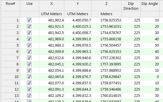
2. Create a new datasheet and enter/import your dip-direction/dip-angle data into the datasheet.
   Or, open one of the sample files and replace that data with your own. (In the Samples folder, an example file = "\RockWorks17 Data\ Samples\Thrust_Fault_Antler_01.rwDat", shown here.) The minimum number of points required to create the fault is 2.

3. Select the Faults | Single Dip List -> Boolean Fault Model menu option.
4. Enter the requested menu settings, described above.
5. Click the Process button to continue. 

The program will read the indicated XYZ location coordinates and create a series of connected panels that are projected up-dip and/or down-dip from the control points, using the Simple or Complex strategy as selected. It will then generate a solid model in which voxels intersected by the fault panels are assigned a "true" value of 1.0. Voxels not intersected are assigned 0.0. The resulting True/false model will be stored on disk under the output solid model file name. If you have requested a diagram, it will be displayed in a RockPlot3D tab.

6. You can adjust any of the input options along the left side of the window and click the Process button again to regenerate the model and display.

   ! Each time you click the Process button, the existing 3D display will be replaced. 

7. View / save / manipulate / print the diagram in the RockPlot3D window. 

Tip: Boolean models contain only two values, such as 0 and 1.  If you want to view only the "true" values (G=1), access the solid model's options (double-click on the Fault Model item in the data listing) and set the minimum all-voxel filter to 0.5.  This will hide all of the 0-value nodes.  

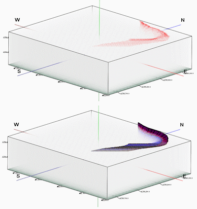
Tip: In RockPlot3D, use File | Append to append a 3D Ribbon Diagram which displays the fault locations with ribbon-like panels.  In the example below, the upper diagram is an all-voxel display of the Boolean model, with transparency applied. The lower diagram shows the fault ribbon appended.

See also: Creating a Boolean Fault Model - Multiple Faults

  Back to Faults Menu Summary

RockWare home page