Tutorial: Create a Lithology Solid Model and Diagram

Estimated time: 6 minutes.

Now we will jump from the Striplogs menu, where we plotted observed data in log diagrams, to the Lithology menu, where the lithology data will be interpolated into a continuous model.

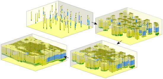
In this lesson, you will create a solid model and 3-dimensional block diagram of lithology. The program will look at the observed lithology intervals, that you viewed in logs and log sections already, and extrapolate the lithology throughout the project, outward from the boreholes. This modeling process basically fills in the blanks between the logs. RockWorks uses a specific lithology modeling algorithm to do this extrapolation. The images below show how you might conceptualize the transformation between observed data which is displayed in logs, and interpolated data which displayed as a solid diagram.

! You must be using RockWorks in Trial mode, or have a Standard or Advanced license to run this modeling program.

Before continuing, be sure you have opened the sample project, established the project dimensions and created 3D logs, as discussed in earlier lessons.

1. With the Samples data still loaded into the Borehole Manager, click on the Lithology menu, and select the Solid option.
   
2. Main Options: These settings will set up the interpolation and diagram settings.
   • Model: Click here to establish the modeling settings:
     
     • Create New Model: Click here to tell the program that we want to interpolate a new solid lithology model (rather than display an existing one). Click this tab to adjust the modeling settings.
       • Solid to be Created: In the Solid Model Output File prompt, type in:     Lithology     . RockWorks will append the .RwMod file name extension for this solid model.
       • 
         
       • Be sure these are not checked:
         • Create Filtering/Resampling Report
         • Limit Input to Selected G Values
         • Limit Model to Selected G Values
         • 
           
       • Algorithm: Click this tab and be sure this is set to Lateral Blending. This is a unique algorithm which "bleeds" lithology types outward from the boreholes into a solid model.
         • Interpolate Outliers: Check this.
         • 
           
       • Special Options: Click on this tab to see all of the options you can adjust for lithology modeling. We won't review all of these at this time. Just be sure these items are checked. The other items can be unchecked.
         • Decluster
         • Smoothing
         • Superface
           • Automatic: Choose this option. The program will automatically create a surface representing the borehole tops (e.g. ground surface) and use this to hide (set to null) lithology model nodes above ground.
           • Buffer Size: Set this to 0.
         • Subface
           • Automatic: Choose this. The program will automatically create a surface representing the borehole bases and use this to hide lithology nodes below the base of the boreholes.
           • Buffer Size: Set this to 0.
           • 
             
   • 3D Solid Diagram: Check this box, and click on this tab to access the diagram settings.
     • Block Diagram: Click this tab.
       • Full Voxel: Choose this option
       • 
         
     • Include Volumetrics: Check this so we'll get volume calculations.
     • 
       
     • Striplogs -> Other 3D Files: Be sure these diagram options are NOT checked.
     • 
       
     • Output Options: Click this tab at the bottom of the listing.
       • Display: Be sure this is checked so that the 3D scene is displayed on completion.
       • Save: Check this to save the diagram in advance.
         • Manual: Choose this and type into the prompt: Lithology Solid. The .Rw3D file name extension wil be appended automatically.
         • 
           
3. Click Continue at the bottom of the window to proceed.

   RockWorks will construct a solid model using the established Output Dimensions. First, it will set those nodes above the ground surface and below the borehole base surface to null. It will then determine the lithology types along each borehole in the project, and assign those nodes along the wells the G value for that lithology as listed in the Lithology Types Table. It will use the lateral blending method to assign lithology to nodes lying between wells. When the model is completed it will be stored on disk under the name Lithology Solid.RwMod.

   The program will read the contents of the lithology solid model file and will create a 3D diagram with all of the lithology zones displayed in a full voxel diagram. The completed diagram will be displayed in a RockPlot3D tab in the Options window.

   ! Note that each time you click the Continue button, the model and/or diagram will be regenerated.

4. Increase the vertical stretch of the display by clicking on the Dimensions button and setting the Vertical Exaggeration to 2.0. Click Apply and then Close.
   
5. View the solid model options: Solid models have some special attributes that you may want to adjust; double-click on the Lithology Model item that is listed in the Data pane.

   

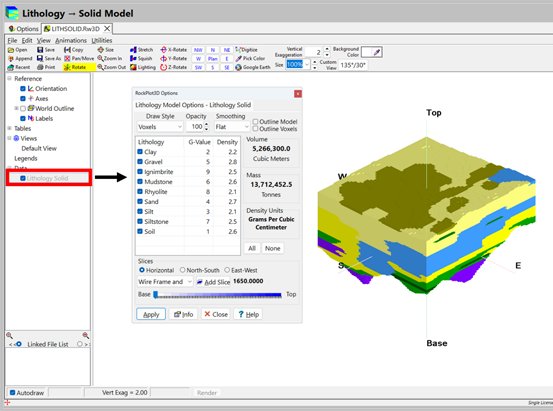
   The program will display a window listing the Solid Model Options. Here’s a quick summary:

   • Color scheme: Since the colors are specific to the colors defined in the Lithology Types Table, RockWorks will list that as source. In other tutorials you’ll see geochemistry solid models displayed differently, such as color-coded from cold-to-hot.
   • Smoothing: Smooth (default) blends the colors in the display while Flat displays abrupt color changes.
   • Draw Style: Default is Voxels. You might try changing the display to Solid (a similar view, but faster to render), Wire Frame or Points to see the effect. Click the Apply button at the bottom of the window to make any changes you set take affect.
   • Opacity: You’ll see this one in most 3D Options windows. You can make the block more transparent by reducing the percent opacity shown here. Again, use Apply to see changes take effect.
   • Filter: This allows you to see only selected G values in the block. See #9 below.
   • Slices: This allows you to see specific slices in the block. See #10 below.
   • 
     
6. If you have a minute, you should go through the next few steps to learn some of the ins and outs of viewing solid model voxel diagrams. If you are in a hurry, you can review these lessons later in the dedicated RockPlot3D tutorial.
   
7. Rotate: Leave the Solid Model Options window open while you Rotate or Pan the image display. (You have full control over the image display even when one or more Options windows are open.) Or, use a viewpoint in the View | Above or Below or Compass Points tools to return to a pre-set view.
   
8. Expand the Lithology Volumetrics heading in the data pane. There you'll see a listing of all of the material types in the project, and their volumes in the current model (see the items circled in blue below). You will also see the G values for each rock type (circled in red) - we'll use this in the next step. You assign a G value for each rock type in the Lithology Types table, and the program uses that value to represent the material in the solid model.

   

   
   
9. Invoke a filter: Click back in the Solid Model Options window.
   1. Filter Enabled: Check this.
      1. In the Low prompt type in 3.0 and in the High type in 5.0, and press Apply to see only those areas where the silt (G=3), sand (G=4) and gravel (G=5) materials are present. If the Show Volume box is checked, the program will display right there in the window the total volume of these materials in the current model.
      2. Try this one more time, changing the Low value to 6 and the High value to 7 and clicking Apply, so that the mudstone and siltstone materials are displayed. You can click back into the image and rotate as you wish for a different view. Note that the Show Volume value is updated to reflect the sand & gravel volume.
         ! In your own work, you may decide to have fewer lithology types, or more, depending on the level of detail you're after. The G values can be grouped by gradational rock types, as they are here, or completely random. The G values can be integers use decimal places.
   2. Filter Enabled: Now, uncheck this. Click Apply.
      
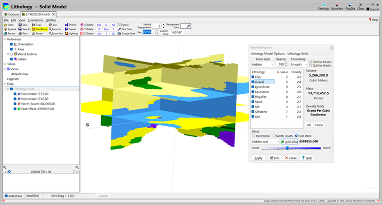
10. Insert some slices: Another means of visualizing the inside of the lithology model is to insert some slice planes.
    1. Horizontal: Click in this button in the Slices section of the window. This tells the program that you want to insert a horizontal slice. The slider bar will show the elevation at the base of the model to the left and the elevation at the top of the model at the right. Drag the slider bar to the right, to an elevation of around 1715, and click the Add button.
    2. The program will insert a slice in the Data listing in the data pane. Hmmm – nothing shows up in the image pane. We need to hide the voxels to see the slice.
    3. Draw Style: Choose Hidden, and click Apply. Aha, there’s the horizontal slice.
    4. Add another horizontal slice by dragging the slider bar to an elevation of 1740 and click the Add button.
    5. Repeat this process if you would like to insert vertical North-South or East-West slices. For these entities, the slider bar will represent south-to-north or west-to-east coordinates.
    6. If you want to remove a slice, right-click on the slice’s name in the Data listing, and choose Delete.

    

11. Close all of the Options windows that may be open, by clicking the Close button in each.
    
12. Save this view: Choose the File | Save menu option. You assigned the name of the RockPlot3D file before it was generated, this will just save the recent changes.
    
13. Append your logs: Finally, if you want to append your 3D strip logs from an earlier lesson to your slice display, choose the File | Append menu option, choose the file Lithology logs.Rw3D and click Open. You will see your 3D strip logs displayed along with the model slices.
    
14. Save this combined view: Choose File | Save, and the new entities will be saved in this view.
    
15. Close this RockPlot3D window by clicking in its upper-right Close box (X).
    

Solid modeling reference, Creating lithology models

  Back to Lithology menu     |     Next (interpolated section) 

RockWare home page