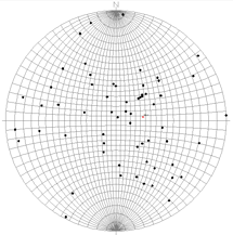
- Projection: Here you can establish how points are to be projected on the stereonet plot, as an equal angle or Wulff projection, or as an equal area or Schmidt projection. A lower hemisphere projection is used for both types.
! NOTE Stereonet contours (activated below) are based on point distributions within a Schmidt projection (equal area) diagram. If you plot points on a Wulff stereonet AND include contours, you may note that the point densities and contours might not correspond.
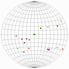
- Symbols: Insert a check here to activate the plotting of symbols on the stereonet. If your data are specified as Lineations, the symbols will represent the point of intersection on the stereonet sphere of the lines. If your data are specified as Planes, the symbols will represent the point of intersection of the poles to the planes. Click on this tab to access the symbol settings.
Symbols are not offered for grid-based stereonet diagrams.
-
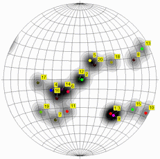
- Labels: Insert a check here to turn on the plotting of labels for each point in the stereonet. Click this tab to access the label settings. Be warned that if there are many samples to be plotted, including individual labels can make the diagram difficult to read. If this is the case, the Diagram Legend (below) can be another way to identify samples.
Labels are not offered for grid-based stereonet diagrams.
-
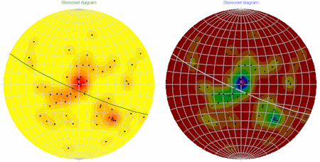
- Contours: Insert a check in this check-box to activate the plotting of line contours on the diagram to represent point density. Click this tab to access the contouring settings. If you request contours, they will be drawn based on a program-computed grid model; be sure you establish the Gridding Options (see below).
-

- Color Contours: Insert a check in this check-box to activate the plotting of color-filled intervals to represent point density on the diagram. Click this tab to access the colorfill settings. As with the line contours, above, the color intervals will be drawn based on a program-computed point-density grid model.
-
- Gridding Options: Click on this tab to establish how the point densities are to be computed if either line or color-filled contours have been requested on the stereonet plot. The program uses a process of "gridding" to compute point densities, in a manner similar to the gridding process for creating maps. However, the methods used to extrapolate the grid node values in a stereonet differ from the methods used in mapping. For "basic" gridding, you might select the Step Function method, with density units in Percent.
- Gridding Method: Choose from Step Function or Spherical Gaussian methods. (More info)
- Density Units: Choose from Standard Deviation or Percent. (More info)
! Stereonet contours are based on point distributions within a Schmidt projection (equal area) diagram. If you plot points on a Wulff stereonet AND include contours, you may note that the point densities and contours might not correspond.
- Title: Check this to activate the plotting of a diagram title. Click on this tab to enter title text, color, size, and position.
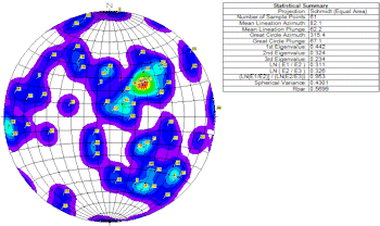
- Statistics : Check this item to plot a statistical legend for the data. Click this tab to establish the legend settings. (More info)
-

- Extras
- Great Circles: Check this item to activate the plotting of planar data as great circles. (If the source data are Lineations, this option will be ignored.)
- Uniform Style/Color: Choose this to display the planar great circles in a constant line style, thickness, and color, which you can select.
- Variable Style/Color: Choose this to choose sample-specific line styles and colors. This requires that you have a column in the current datasheet where these are defined. Select that column name.
-

- Mean Lineation Vector: Check this to plot the mean lineation vector. Select a symbol to represent it on the plot, a color for the symbol, and the label.
-

- Best Fit Circle: Check this to plot the program-computed best-fit great circle on the stereonet. Select its line style and color.
- Background: Click this tab to turn on and off a variety of reference lines, ticks, and labels.
- Style/Width/Color: Click on this box to select the style, thickness, and color of the lines to be displayed in the background grid.
- Perimeter: Check this item to include a solid-line perimeter circle. (Recommended)
- Tick Marks: Check this to plot small tick marks on the top, bottom, left, and right sides of the perimeter circle.
- North Arrow: Check this box to include the letter "N" at the top of the diagram.
- Schmidt/Wulff Net: Check this to plot background lines specific to Schmidt or Wulff nets. (The program will pick the right one for the Projection you specified, above, under the Projection heading.)
- Spacing: Choose the desired background grid spacing. The examples below illustrate 5-degree and 10-degree Wulffnets.
-

- Lambert Equal Area Net: Check this option to include azimuth lines/dip circles for Lambert projection lines.
- Azimuth Lines: Check this to plot the radial spoke lines. Click to the right to specify the degree spacing for the lines.
- Dip Circles: Check this to plot the concentric dip circles. Click to the right to specify the dip degree spacing for the lines.
RockWare home page