Creating Stereonets

RockWorks | Utilities | Planes | Stereonet Diagram

This program reads planar, linear, or rake data from the data sheet, and displays the orientation of these features on a stereonet diagram in RockPlot2D using points and great circles. Optional gridding is available to display point density with line or color-filled contours. Equal angle and equal area projections are available.

Menu Options
Step-by-Step Summary

Menu Options

• Input Columns: The prompts along the left side of the window tell RockWorks which columns in the input datasheet contain what data.
  Click on an existing name to select a different name from the drop-down list.
  • Direction: Select the datasheet column that contains the strike bearing or dip direction. 
    ! Be sure you correctly identify the input data type under Data Type, below.  
  • Dip: Select the column that lists the dip angle, in degrees, where 0 = horizontal and 90 = vertical, downward. 
  • Rake Angle: If the input data type is set to Rakes you must also specify the data column that lists the rake angle.
     
• Input
  • Data Type: In the middle pane of the window, choose what the data listed in the data sheet represents.
    • Planes: If you choose Planes, the program will represent the data on the stereonet as poles to planes (if Symbols are activated) or as great circles (if Great Circles are activated). 
    • Lines: Samples will be represented using symbols.   
    • Rakes: Samples will be represented using symbols.  Be sure that the Rake Angle data column is specified in the left-hand 
      pane.
  • Data Convention: Choose how the planar data listed in the data sheet is recorded.
    • Right Hand Rule: Using this convention, planar data is entered as strike bearing and dip angle, with the 
      dip direction being 90 degrees clockwise from the strike azimuth bearing.
    • Dip Direction: Using this convention, planar data is entered with dip direction and dip angle.
      
      
• Stereonet Options (See the Details topic for more information about these stereonet-specific settings)
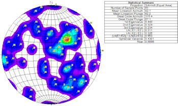
  • Projection: Determines how points are to be projected on the stereonet plot, as an equal angle or Wulff projection, or as an equal area or Schmidt projection. A lower hemisphere projection is used for both types.
    ! Note Stereonet contours (activated below) are based on point distributions within a Schmidt projection (equal area) diagram.  If you plot points on a Wulff stereonet AND include contours, you may note that the point densities and contours don't correspond.
    
    
  • Symbols: Insert a check here to activate the plotting of symbols on the stereonet. If your data are specified as Lineations, the symbols will represent the point of intersection on the stereonet sphere of the lines. If your data are specified as Planes, the symbols will represent the point of intersection of the poles to the planes. Expand this item to access the symbol settings. 
  • Labels: Insert a check here to turn on the plotting of labels for each point in the stereonet. Expand this item to access the label settings. Be warned that if there are many samples to be plotted, including individual labels can make the diagram difficult to read. If this is the case, the Diagram Legend (below) can be another way to identify samples.
    
    
  • Contours: Insert a check in this check-box to activate the plotting of line contours on the diagram to represent point density. Expand this item to access the contouring settings. If you request contours, they will be drawn based on a program-computed grid model; be sure you establish the Gridding Options (see below). 
  • Colored Intervals: Insert a check in this check-box to activate the plotting of color-filled intervals to represent point density on the diagram. Expand this item to access the colorfill settings. As with the line contours, above, the color intervals will be drawn based on a program-computed grid model.
  • Great Circles: Use this check-box and it settings to activate the plotting of planar data as great circles. (If the source data are Lineations, this option will be ignored.) Expand this item to select the line styles.
    
    
  • Mean Lineation Vector: To activate the plotting of the mean lineation vector, insert a check in this box. Expand this to select a symbol to represent it on the plot, and the label
  • Best Fit Circle: Insert a check in this box to activate the plotting of the program-computed best-fit great circle on the stereonet. Expand this item to select its line style and color.
    
    
  • Title: Check this to activate the plotting of a diagram title, and expand this to enter the text, color, size, and position.
  • Statistics : Check this item to plot a statistical legend for the data. Expand this item to select text size and color.  (More.) (See also the Statistical Summary.)
  • Background: Expand this heading to turn on and off a variety of reference lines, ticks, and labels. (More.)
  • The Gridding Options and Density Units items in the Stereonet Options window are used to establish how the point densities are to be computed if either line or color-filled contours have been requested on the stereonet plot. The program uses a process of "gridding" to compute point densities, in a manner similar to the gridding process for creating maps. The methods used to extrapolate the grid node values in a stereonet differ from the methods used in mapping, however. To access these settings, expand the Gridding Options item.  For "basic" gridding, you might select the Step Function method, with density units in Percent. See Stereonet Gridding Options for a lengthy explanation.
    ! Note Stereonet contours are based on point distributions within a Schmidt projection (equal area) diagram.  If you plot points on a Wulff stereonet AND include contours, you may note that the point densities and contours might not correspond.
     

Step-by-Step Summary

1. Access the Utilities program tab.
2. Create a new datasheet and enter/import your strike and dip data into the datasheet.
   Or, open one of the sample files and replace that data with your own. (In the Samples folder, an example file = "\RockWorks17 Data\ Samples\Strike_and_Dip_Map_01.rwDat".) The Stereonet program can process a single point for diagrams, but requires at least three points for statistical calculations.
3. Select the Utilities | Planes | Stereonet Diagram menu command.
4. Enter the requested menu items, described above.
5. When all of the stereonet settings are established to your satisfaction, click the Process button at the bottom of the window.

The program will read the measurements from the data sheet and create the stereonet plot, including the requested items. The completed diagram will be displayed in a RockPlot2D tab in the Options window.

6. You can adjust any of the settings in the Options window (diagram settings, etc.) and then click the Process button again to regenerate the stereonet.
   ! Each time you click the Process button, the existing display will be replaced. 
    
7. View / save / manipulate / export / print the map in the RockPlot2D window. 
   
   

  Back to Planes Menu Summary

RockWare home page