Creating Vector (Cavern) Models

RockWorks | Borehole Manager | Vectors | Model

Use this program to:

• Create a new 3-dimensional solid or block model (an .RwMod file) that approximate the extents of the vectors stored within the Vectors table - OR - read an existing .RwMod file you've already created.
• Display the vector model as a 3D voxel diagram in RockPlot3D.

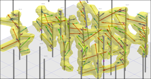
An example application is the generation of void geometries (cave models) based on downhole laser surveys. 3D logs can be included. The completed diagram will be displayed in a RockPlot3D window, where there is a variety of filtering and visualization options. 

Feature Level: RockWorks Standard and higher

Menu Options
Step-by-Step Summary
Tips

Menu Options

• Cave Model: First, tell the program whether you wish to use an existing solid model (from a previous use of this tool) or you wish to create a new solid model, by clicking in the appropriate radio button.
  ! NOTE This is not trivial. Creating the solid model can take some time, depending on the resolution of the model and the detail of your data. If you already created a pleasing model, and simply wish to create a new 3D view of it, you can select the same model, which was stored on disk as an .RwMod file, for the solid or isosurface model.
  • Create New Model: If want to create a new model, click in this radio button, and expand this item to establish the modeling settings.
    • Solid Model Name: Click to the right to enter a name for the solid model, with an .RwMod file name extension.
    • Model Dimensions: Expand this item to set the model density. (More.)  For cave models this can be tricky. If you make the cells too small, the model will look very tubular. If you make them too large, you lose resolution. Experimentation is therefore necessary. In general, a good starting point is to make the cell width equal to half of the average minimum spacing between the boreholes. 
      • You can expand the Hardwire Output Dimensions options to view the existing settings and adjust them as necessary.
      • You can choose Variable (Data Specific) Dimensions and turn on the Confirm Model Dimensions option to view the settings prior to interpolation.
    • Negate Node Values: If left unchecked, the node values will represent the distance to the closest vector. When plotting the output as an isosurface, the cutoff level (and slider bar) will behave in a fashion that is opposite to what you'd expect (i.e. the voxels closer to the vectors will be rendered invisible). The "Negate Node Values" will multiply all of the voxel g-values by -1 such that the g-values become higher with proximity to a vector. This allows the cutoff level to behave as you might expect.
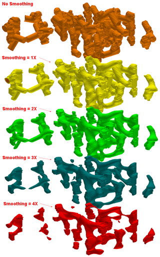
    • Smooth Solid: This will effectively round-off the edges of the "tubes" and create a more natural appearance. Be careful, however, with too much smoothing. Notice how the 4X smoothing (filter size = 1x1 for all models) within the following diagram has removed some salient features.

  • 

  • Use Existing Model: Click in this radio button if you wish to use an already-existing solid model of your interval data.  Expand this item to select: 
    • Model Name: Click to the right to browse for the name of the existing solid model (.RwMod file) to be used for this solid or isosurface diagram. 
       
• Create Solid Diagram: Insert a check here to display the new or existing solid model as a 3D diagram.  Expand this heading to establish the diagram options.

• Diagram Type: Choose from one of the following. (More.)
  • All Voxels: Click in the All Voxels radio button to represent the solid model in the 3D display as color-coded voxels.  You can choose to display either the Full Voxel, or just the Midpoint.  Display of the midpoint only can significantly improve display time for huge models.
    ! Note: You can toggle between Full Voxels and Midpoints in RockPlot3D after the model is displayed.  For this reason, if you're interpolating/displaying a large model, choose Midpoints; should you later prefer to view the full voxel image, you can select this in the display window itself.
  • Isosurface: Click in the Isosurface radio button to display the solid model as if enclosed in a "skin."  This view will be smoother than a voxel display, and is the recommended viewing style for cavern models.
    
    
• Iso-Mesh: Check this box to include mesh lines around the isosurface diagram.  Expand this heading to set up the iso-mesh cutoff, line style, etc.  (More.)
  
  
• Plot Logs: Check this box to append striplogs to your 3D diagram. 
  • Clip Logs: Check this sub-item if you want to restrict the logs to a particular elevation range. 
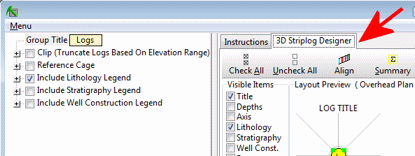
  • 3D Striplog Designer: Click on the 3D Striplog Designer tab to the right, to select the items to display in the individual logs to plot with the model.

  • 
     

  • • Visible Items:  Use the check-boxes in the Visible Items column to select which log items are to be displayed.  See Visible Item Summary for information.
    • Options: Click on any of the Visible Items names to see the item's settings in the Options pane to the right.  See Visible Item Summary for links to the Options settings.
    • Layout Preview: For each item you've activated, you'll see a preview cartoon in the upper pane, showing an overhead view of the log columns.  Click and drag any item to rearrange the log columns; click and drag the circle handles to resize a column.  See Using the 3D Log Designer.
      
      
• Diagram Title: Type in the title for the diagram, which will be displayed in RockPlot3D.
  
  
• Color Scheme: Click on the Options button to define the display's color scheme - automatic, table-based, etc. (More.)
  
  
• Reference Cage: Insert a check here to include vertical elevation axes and X and Y coordinate axes in the 3D diagram. Expand this item to set up the cage items.  (More.)
  
  
• Include Legend: Insert a check here to include an index to the colors and G values in the diagram.  (More.)

Step-by-Step Summary

1. Access the RockWorks Borehole Manager program tab. 
2. Enter/import your data into the Borehole Manager. This tool specifically reads location, orientation (if any), and Vector data. The distance measurements would be recorded in the Value column.

3. Select the Vectors | Model menu option. 
4. Enter the requested menu settings, described above.
5. Click the Process button to proceed. 

If you've selected Use Existing Model, the program will load the information from the existing model (.RwMod file), and will proceed to diagram generation.

If you've selected Create New Model, the program will scan the project database and extract the XYZ points for all of the downhole vector measurements.

6. If you have requested model confirmation, the program will display a window at this time.  Adjust these dimensions as necessary and click OK to continue.  (More.) 

This program will perform the following operations in order to generate a model that approximates cave geometries based on the vector data:
For each solid model node ...
   For each borehole ...
      For each vector ...
            Compute the endpoint coordinates.
            Define a line connecting the endpoints.
            Define a sphere whose center is defined by the line midpoint and whose diameter is equal to the line length.
            If the node resides outside of the sphere its g-value is set to "null" (-1.0E27).
            If the node resides inside of the sphere, its g-value is set to the distance to the closest line.

Note: In order for the node values to increase with distance to the closest line, it is necessary to negate the distance values (i.e. the node values should be multiplied by -1) as allowed within the Vector Modeling Options menu.

The completed model will be stored under the indicated .RwMod file name. 

If you requested a diagram, the model will be displayed in a RockPlot3D tab in the Options window, using the using the requested display type. If you activated the Plot Logs feature, the program will also append the 3D logs to the diagram.

7. You can adjust any of the following items and then click the Process button again to regenerate the display.
   • Vector model settings in the Options pane on the left*, and/or
   • Diagram settings in the Options pane on the left, and/or
   • Striplog settings in the 3D Striplog Designer tab.

   ! Each time you click the Process button, the existing 3D display will be replaced. 
   ! * If the solid model looks OK and you just need to adjust one of the diagram settings, you don't need to keep re-interpolating the model.  Choose Use Existing Model and browse for the .RwMod file to be used for the 3D view.

8. View / save / manipulate / print / export the model in the RockPlot3D window. 

Tips:

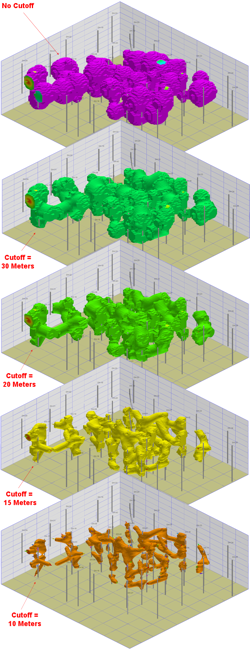
1. Once the modeling process has been completed, the initial diagram will be displayed in which the cave appears as a series of coalescing spheres. Experiment with the isolevel setting. During this process, notice how a highly filtered model will generate tubes around the laser paths. As a consequence, it is necessary that various cutoff levels be applied to achieve the desired diagram (e.g. cutoff = 25 meters).  Note: If the "Negate Node Values" option was activated prior to the generation of the model (which it should have been), you will need to enter the isosurface cutoff value as a negative number.

2. Change the opacity/transparency level of the isosurface to 50% in order to see into the model and compare the model with the original vector data.
   Save this diagram as "Caves.Rw3D".
   
3. Convert the distance-to-point model to a boolean model by selecting the Utilities | Solid | Boolean Operations | Boolean Conversion option.

   
   

   • In order to use this program, you must enter the minimum distance as the lower threshold (cutoff) value. Let's say that you specified -20. Any voxels that are less than 20 meters from a vector will be set to a value of 1 (true) while any voxels greater than 20 meters from a vector will be set to zero (false) within the new, boolean model. The net result can be interpreted to mean that nodes with a value of 1 represent voids whereas nodes with a value of 0 represent rock.
     
     
   • Remember that the distances within the model are expressed in negative values (assuming that you chose to "Negate" the values when the model was initially created). The high-cutoff won't be used, so specify something ridiculously high like 9999.
     
     
   • Name the new, output model "Boolean.RwMod".
     
     
   • A diagram of the boolean model will look very similar to the original, continuous cave model. It's just more blocky and doesn't have the low values.
     
     
4. Convert the boolean model into a grid model by selecting the Utilities | Solid | Convert | Solid -> Grid option.

   
   

5. • Be sure to check the "Sum" option within the Solid->Grid menu. This means that the grid nodes will be defined as the sum of all nodes within the corresponding solid model vertical column. Given that a voxel value of one within the boolean model represents a void, a grid node value of five would mean that five nodes below that cell are void.  
     
     
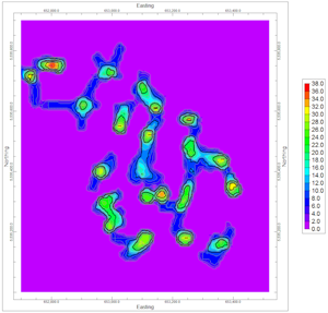
   • The map of this grid shows, in a continuous fashion, the areas that are most dangerous for heavy equipment. Admittedly, it does not take into account the depth of the caverns (e.g. a large, but very deep cavern may be of no concern).

   

5. Use the RockPlot2D | Export | RockPlot3D option to create an overlay of the contour map to show in conjunction with the 3D model.
   • In order to "see through" this layer into the solid model, we recommend that you plot only the contours rather than a color-fill map.
     
     
6. Once the diagram has been displayed within RockPlot3D, save it as "Contour Overlays.Rw3D".
   
   
7. Use the RockPlot3D | File | Append option to append the caves diagram (caves.Rw3D) and the boreholes (boreholes.Rw3D).

Back to Borehole Manager Summary

RockWare home page