Tutorial: Create a T-Data Model and Isosurface Diagram

Estimated time: 5 minutes.

Now we will jump from the Striplogs menu, where we plotted observed data in log diagrams, and the Aquifers menu, where we interpolated water surface models, to the T-Data menu, where the downhole quantitative data will be interpolated into a continuous solid model.

In this lesson, you will create a solid model and 3-dimensional isosurface diagram of the project's Toluene measurements, for a specific date. The program will load the recorded borehole data, that you viewed in logs and log sections already, and extrapolate the measured values throughout the project. This modeling process basically fills in the blanks between the boreholes. RockWorks offers several modeling algorithms to do this extrapolation; sparse time-based data typically requires a different modeling technique than denser data might.

Before continuing, be sure you have opened the sample project, established the project dimensions,  created 3D logs, and created an aquifer model as discussed in earlier lessons.

1. With the Samples data still loaded into the Borehole Manager, click on the T-Data menu, and select the Solid option..
   
2. Main Options: These settings will set up the interpolation and diagram settings.
   
   • Model: Click here to establish the modeling settings:
     
     • Create New Model: Click here to tell the program that we want to interpolate a new T-Data model (rather than display an existing one). Click this tab to adjust the modeling settings.
       • Solid to be Created: In the Solid Model Output File prompt, type in:     Toluene 2-14-17     RockWorks will append the .RwMod file name extension for this solid model.
       • 
         
       • T-Data Track: Click here to select from the pop-up list the column titled Toluene. Be sure that none of the options below that (filters, resampling) is turned on.
         ! Note how you've included the date in the model name - this can be handy to keep track of which solid model represents which date measurements. RockWorks does not assign these names automatically.
       • 
         
       • Algorithm: ! For Time Interval Data, this is important. The default method that RockWorks uses for general solid modeling is Inverse Distance Anisotropic. While this works well for numerous I-Data measurements, this isn't the best choice for the limited measurements typical of T-Data.
         • IDW Advanced: Click in this radio button; note that modeling options are displayed to the right.
           • Weighting Exponents: These options allow you to vary the influence of measurements that lie horizontally versus vertically in relation to each node being interpolated. The greater the exponent value, the less influence the measurements will have.
             • Horizontal: Set this exponent to 2. (normal influence)
             • Vertical: Set this exponent to 4. (reduced influence)
           • Search Method:
             • All Points: Choose this option so that the program will not limit the search for measurements to consider when interpolating the node values.
               
       • Special Options:
         
         • Decluster: Unchecked.
         • Smoothing: unchecked.
         • Cutoff - H, Cutoff - V: unchecked.
         • Add Points: unchecked.
         • Logarithm: unchecked. If used, this can be helpful for interpolation of highly anomalous data.
         • HiFi: unchecked.
         • Distance: unchecked.
         • Polygon: unchecked.
         • Superface: Check this to activate an upper surface (grid) filter, and click on the tab to access the settings.
           • Manual: Click on this option to the right. While Automatic filtering works well for many project-wide solid models, we want to constrain this model with the water level surfaces created in the previous lesson.
             • Grid Model: Click here to browse for the file "Aquifer 1_2_14_2017_top.RwGrd". (Your file name may have a different date order.)
           • Buffer Size: Set this to 0.0.
         • Subface: unchecked.
         • Tilting: unchecked. If activated, this can be used to apply a tilt to the model.
         • Warping: unchecked. If activated, this can be used to warp a model based on a surface.
         • Faulted: unchecked. If activated, you can use a 3D "fault file" to introduce faults into your model.
         • G=Color: unchecked. This is used for color modeling only.
         • Constrain: unchecked. This is used for limit modeling to defined areas within a Boolean model.
         • 
           
         • Dimensions: These define the extents of the output model.
           • Based on Output Dimensions: Be sure this option is checked.
           • Confirm Model Dimensions item can be left unchecked (though in your own work, this is a handy way to double-check the model extents and node spacing).
           • 
             
         • Undefined Nodes: Use this setting, at the bottom of the window, to define the value to be assigned to the solid model nodes above the water level top and below the water level base. (All project nodes are present in the model; "filtered" nodes can be set to a specific value to "hide" them.)
           • Null (-1.0e27): Choose this option.
           • 
             
   • Create 3D Diagram: Check this, to tell RockWorks that you want to create a 3D diagram to represent the solid model. Click this tab to access the diagram settings.
     • Block Diagram: Click on this tab.
       • Isosurface: Choose this - it will create a diagram in which the different G value levels can be represented as if enclosed within a "skin" that is like a 3-dimensional contour. Within RockPlot3D you can interactively adjust the minimum T-data value to be enclosed within the isosurface contour.
         • Include IsoMesh: Uncheck this.
       • Filter: Unchecked.
       • Color Scheme: This should default to a continuous cold-to-hot 2-color scheme. In your own work, if you want to display specific concentrations using specific colors you can use the Custom option, for which you create a table that lists G value ranges and the colors to represent them. Note that the color scheme can also be adjusted once the isosurface is displayed in RockPlot3D.
       • 
         
     • Striplogs: Check this. RockWorks will generate the 3D logs using the same settings we used in an earlier lesson in this section.
     • 
       
     • Draped Image: Unchecked.
     • Floating Image: Unchecked.
     • 
       
     • Perimeter Cage: Insert a check in this box and click on the tab to see the options.
       • Dimensions: This should be set to the Automatic.
       • Panels: Click on this tab and be sure these are all unchecked.
       • Grids: Click on this tab and be sure that all of these are also unchecked.
       • Axis Labels: Click on this tab and check these options only; you can refer to the cartoon for a preview.
         • Southwest
         • Base / East
         • Base / South
         • 
           
     • Legends: Check this item and click on the tab.
       • Color: Choose this legend type.
       • 
         
     • Infrastructure: Unchecked.
     • Faults: Unchecked.
     • Other 3D Files: Unchecked.
     • 
       
   • Output Options: Click on this tab.
     • Display: Be sure this is checked, so that the 3d scene will be displayed on completion.
     • Save: You can leave this un-checked. We will save the file once it is generated and displayed.
     • Export: Be sure this is not checked.
     • 
       
3. Now move to the tabs at the top of the window.
   • Spatial Filter: Unchecked.
   • Time Filter: Be sure this is checked, and still set to Feb 14, 2017.
   • 3D Log Design: This should still be set to display T-Data Toluene logs, from a previous lesson.
   • 
     
4. Click the Continue button at the bottom of the T-Data Model window. RockWorks will create two items:
   
   It will interpolate a solid model using the specified project dimensions using the IDW Advanced method of extrapolating the Toluene concentrations for those areas with no boreholes, using the date-filtered input data. Nodes which lie above the constraining water surface will be assigned a Null value. The completed model will be stored in the project folder with the name Toluene 2-14-17.RwMod.
   
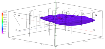
   RockWorks will then create an isosurface diagram to illustrate the model. The completed diagram will be displayed in a RockPlot3D tab.
   
5. View the isosurface model options by double-clicking on the Toluene item that’s listed in the data tree.

   

   The program will display a window listing the Isosurface Options. Here’s a quick summary:

   • Color scheme: This solid model contains G values representing Toluene concentrations that range from a minimum to a maximum. The default scheme will be set to Continuous, to show continuous gradations between the low and high values. If you wish, you can change the by clicking on the Min-Max button to the right of the color scheme. In your own work, if you want to display specific concentrations using specific colors you can use the Color Table option, for which you create a table that lists G value ranges and the colors to represent them.
   • Draw Style: Default is Solid. You might try changing the display to Wire Frame to see the effect. Click the Apply button at the bottom of the window to make any changes you set take effect. Using Wire Frame can speed rendering of the solid if it is dense or your computer system is slow.
   • Opacity: You’ll see this one in most 3D Options windows. You can make the block more transparent by reducing the percent opacity shown here. Again, use Apply to see changes take effect.
   • Plot Outline: This draws an outline around the boundary of the model.
   • Cap Style: This tells the program how you want the portions of the isosurface that intersect the edge of the model to be displayed. By changing the contour interval, you can see how the concentrations change inside the isosurface.
   • Iso-level: This allows you to see only selected G values in the block. See #6 below.
   • Slices: This allows you to see insert horizontal or vertical slices at specific locations in the block.

   If you have a minute, you should go through the next few steps to learn some of the ins and outs of viewing isosurface diagrams. If you are in a hurry, you can review these lessons later in the dedicated RockPlot3D tutorial.

6. Change the iso-level being displayed: Find the slider bar in the Iso-Level section. The left-hand value on this slider corresponds to the minimum Toluene concentration in the model, and the right-hand value represents the maximum concentration. Drag the slider bar slowly to the right, with the intention of changing the minimum Toluene level displayed, to see how the display changes. In your own work you can use the slider or just type a minimum desired value into the prompt. Try typing:  40   into the Iso-Level Value prompt and clicking Apply.
   
   Note that you can Rotate or Pan the image at any time without closing the Options window to get a better view. Or, use the View | Above, the View | Below, or the View | Compass Points tools to return to a pre-set view.
   
7. Show the current volume: Insert a check in the Show Volume check-box and the program will display right in the Options window the total volume in the model at the minimum Toluene concentration and above. If you drag the slider bar to change the minimum isosurface level, the volume will change.
   
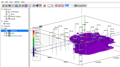
8. Adjust the transparency: To see through the isosurface to the logs inside, which represent the observed data values, set the Opacity value to 70 and click Apply.

   

9. Save the current scene: Choose File | Save and type in this name: Toluene 2-14-17
   RockPlot3D will append the .Rw3D file name extension automatically.
   
10. Close this RockPlot3D window by clicking in its upper-right Close box (X).
    

Solid Modeling Reference, Creating T-Data Models
 

  Back to T-Data menu     |     Next (interpolated cross section) 

RockWare home page