 Estimated time: 2 minutes.
The Ternary command in the Stats menu is used to create a ternary plot for three variables read from the main datasheet. We will use a different sample file than we used in the earlier lessons of this section.
- Be sure you’ve accessed the RockWorks Utilities datasheet and opened the Samples project folder.
- Open a new sample file:
- In the Project Manager pane along the left edge of the program window, expand the Datasheet File heading if necessary.
- Look for the file named Soil_Properties_01.RwDat.
- Double-click on that file name to open it.
- If you are prompted to save changes to the existing datasheet, click No.
The program will display this file in the main Utilities datasheet. This data set contains an ID, symbol, X and Y location coordinates, and elevation for each sample site. It then lists sand, gravel, and clay percentages, Ca and Mg measurements, several geotechnical measurements, and soil colors. For this exercise, we will display the sand/gravel/clay components in the ternary plot.
- Select the Ternary | Single option from the Statistics menu.
- Input Columns: Use these prompts along the left to establish data setup. The name of the currently-selected datasheet column for each required input field is displayed below each prompt. To change a column name for any of the prompts simply click on the small down-arrow and select another column name. The prompts and column names you need to establish are listed here:
- Upper Vertex: Set to the column named Sand for the data to be represented in the upper vertex in the diagram.
- Left Vertex: Set to the column Gravel for the data to be represented in the lower-left vertex in the diagram.
- Right Vertex: Set to the column Clay for the data to be represented in the lower-right vertex in the diagram.
- Titles: Expand this heading to establish the diagram and axis titles. (These may already be displayed as defaults.)
- Primary: Click here and type in: Sand/Gravel/Clay Distribution and click OK.
- Secondary: Click here and type in: Site 27B and click OK.
- Vertex Labeling: Expand this option and set the vertex titles as shown:
- Upper Vertex: Sand
- Left Vertex: Gravel
- Right Vertex: Clay
- Symbols & Contours: Click the Options button to the right.
 Symbols: Check this option.
 Uniform: Uncheck this.
 - Column-Based: Check this option.
- Symbol Column: Click here and choose the "Symbol" column.
- Dimensions: Choose Uniform, at a size of 3.0.
- Circles: Uncheck this.
- Table-Based: Uncheck this.
- Images: Uncheck this.
- Symbol Labels: unchecked
- Contour Lines: unchecked
- Colored Intervals: unchecked
In your own work you may want to include point labels, if your data set is not this large. You may also want to request line and/or color-filled contours to illustrate point density.
- Click OK to close the Options window.
- Gridding Method can be ignored since you have not selected any contouring.
- Annotations & Embellishments: Click on the Options button to the right.
- Subdivisions: Click on this item.
- Major Subdivisions: Check this option. Click on the Line Styles sample to select thin, black lines.
- Minor Subdivisions: Be sure this is checked. Click on the Line Styles sample to select thin lines, and set the color to light gray.
- Intervals: Choose Major = 10% / Minor = 2%
- Perimeter: Check this option.
- Axis Labeling: Check this option, and click on the tab to choose 20% for the interval.
- Tick Marks: Check this option, and choose 20% for Increments and Internal for the locations.
- Classification Overlays: Un-check this. These new options will plot a pre-defined diagram in the background with your data points and/or contours in the foreground. The currently available templates include Folk's (1954) siliclastic classification system, Schlee's (1973 - after Shepard) siliclastic classification system, Shepard's 1954 siliclastic classification system, and the USDA soil classification system.
- Click OK to close the Annotation & Embellishment Options window.
- Click the Process button at the bottom of the Ternary Diagram window to proceed.
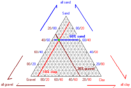
The program will read the values from the Sand, Gravel, and Clay data columns. Each sample will be normalized such that the three components add up to 100%. The symbol for that sample will be plotted at that point in the diagram, with 100% sand represented at the top, 100% gravel represented at the left vertex, and 100% clay at the right vertex.
In the example below, the single sample contains 60% sand, 30% shale, and 10% clay.
- Close this window by clicking the Close button (
 ). Answer No to the save-file prompt.
 Ternary Diagrams
 Back to component menu | Next (pie chart map)

RockWare home page