Tutorial: Create an I-Data Fence Diagram

Estimated time: 4 minutes.

In this lesson, you will create a fence diagram view of the I-data model created back in the I-data model lesson and also illustrated in the previous lesson.  The fence diagram differs from the cross section in two ways: It can contain discontinuous (un-connected) slices of the model, and the output diagram will be displayed in the RockPlot3D window.

The instructions below are written with the assumption that you have completed the 3D logs lesson and the I-data model lesson.

1. Back at the Borehole Manager, click on the I-Data menu and select the Fence option.
    
2. Establish the modeling settings:
    Use Existing Model:  As we discussed in the previous lesson (I-Data | Section), you've already created the model that represents the I-Data, and you can use that model for the fence diagram display. It is not necessary to reinterpolate the model just to create a new diagram. Expand this item.
   Model Name: Click here to browse for the file "benzene soil.RwMod".
    
3. Establish the diagram options:
   1. Color Scheme: Click the Options button and choose a 2-Colors (Min-Max) scheme. You can select a predefined min-max scheme by clicking on the color bar or on the down-arrow on the right side of the long bar. Or, you can choose your own min-max colors by clicking on the single-color boxes on either end. Click OK to close this window.
   2.  Include Color Legend: Check this.
   3. Plot Outline Around Each Panel: Uncheck this.
   4. Plot Surface Profile: Uncheck this.
   5. Plot Logs: The program will generate the 3D logs using the same settings we used in an earlier lesson in this section.
   6. Reference Cage: Uncheck this.
   7. Create Separate Location Map.  Check this, to display your fence panel arrangement in plan-view.
       
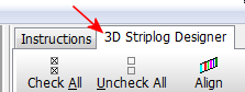
4. Click on the 3D Striplog Designer tab if you'd like to review the striplog setup.
   
   
    
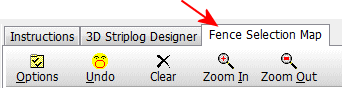
5. Click on the Fence Selection Map next, to define the layout of the fence panels.
   
   

Unlike profile diagrams, fence diagrams permit multiple panels to be selected. These can be drawn in several ways:

• Interactively by you, by clicking the beginning and ending points of the panels, just like you drew the cross section slices, and/or
• Using pre-set panel selections, offered in the buttons to the left, and/or
• From coordinates listed in an "X Y Pairs" table in the database.

For this tutorial, we will use the second option.

6. Select the preset Fence Panels:
   1. Clear: Click on the Clear button at the top, to remove any existing panels.
   2. Snap: Clear this box (upper-left). This allows the panels to be drawn anywhere within the model, not just between boreholes.
   3. Click on the N & S button, to the left.  The program will draw horizontal lines along the north and south borders of the project.
   4. Click on the E & W button. You will see vertical lines drawn along the western and eastern borders of the project.
   5. Click on the Cross button. The program will add north-south and east-west panel lines to the map window.

   

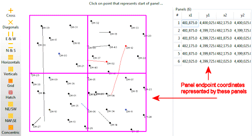
   In your own work, you can use any combination of hand-drawn and/or pre-set panel configurations. If you wish to erase the current panels to re-draw, simply click the Clear button to clear the display.
   ! Because the I-Data model is continuous, you can place the fence panels anywhere within the model - you don't have to place the panel endpoints at the borehole locations.

7. Click the Process button at the bottom of the I-Data Fence Diagram window to continue.
   
   The program will read the contents of the existing, already-saved benzene solid model file and will create vertical slices through the model along the indicated panel lines. The completed diagram will be displayed in a RockPlot3D tab. Three-dimensional logs will be appended to the fence diagram.  The image is displayed in the pane to the right, and the image components as well as the standard reference items are listed in the pane to the left.
   
   The Fence Location map will be displayed in a separate Rockplot2D tab.
    
8. Expand the Benzene Soil Fence item in the Data listing. Note that the 6 vertical panels are listed there. Each can be expanded, where the vertical grid model is listed. (If you can’t tell which panel name corresponds to which panel in the view, remove a check-mark and see which one disappears.)
    
9. Adjust the display as you wish using the Rotate and Pan buttons.
    
10. Adjust the panel opacity: You can adjust the opacity of an entire group of objects (such as the fence panels) by double-clicking on the Benzene Soil Fence group item. Set the Opacity setting to 70 and click Apply. You should now see the logs better. Close the transparency window.
     
11. Turn data items on and off: Take a moment to experiment with turning display items on and off, using the check-boxes in the Data listing in the data pane.
     
12. Save this image: Select the File|Save As command. In the displayed window, type in this name: idata logs+fence and click the Save button. RockPlot3D will save this combined information on disk under that name, with an ".Rw3D" file name extension.
     
13. Close this plot window by clicking in the Windows Close button in the upper-right corner.
    
    

This is the end of the tutorial for interval-based data. The next section contains lessons for time-based interval downhole data.

  I-Data Fences

  Back to I-Data menu       |      Next (T-Data Diagrams) 

RockWare home page