Modeling Fractures in Three Dimensions

RockWorks | Utilities | Solid |
Fracture Disks -> Solid

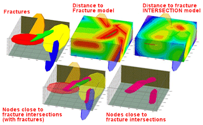
This program is used to create a solid model from fracture locations, assigning voxel values based on the distance between a voxel node and the closest point on the closest disk, or between the voxel and the closest fracture intersection.  These disks are meant to represent fractures.  This is the same tools as in the Borehole Manager Fractures | Model option, but reads the measurements from the Utilities datasheet.

Possible applications include:

• Hydrology: Fractured Aquifers
• Mining: Hydrothermal Conduits
• Petroleum: Fractured Reservoirs
• Geotechnical:  Site Excavations / Slope Stability

Menu Options
Step-by-Step Summary
 

Menu Options

• Data Columns
  • X-Column:  Defines the datasheet column that contains the easting coordinates at the center of the fracture disks.
    ! The coordinates can be in the project coordinate system or another system. See Defining your Datasheet Coordinates for more information.
  • Y-Column:  Defines the datasheet column that contains the northing coordinates at the center of the fracture disks.
  • Z-Column:  Defines the datasheet column that contains the elevations at the center of the fracture disks.
  • Direction Column:  Defines the datasheet column that contains the dip-directions for the fracture disks.
  • Dip Angle Column:  Defines the datasheet column that contains the dip-angles for the fracture disks.
  • Radius Column:  Defines the datasheet column that contains the radii for the fracture disks.
     
• Output File: Click to the right to type in the name for the solid model (.RwMod file) in which to store the numerical solid model.  
  
  
• Model Dimensions: Expand this item to set the model density. (More.)
  
  
• Type of Model: Use these settings to define the type of frature model to be created:
  • Distance to Closest Fracture: This algorithm assigns block model node values that represent the distance to the closest frature.
  • Distance to Closest Fracture Intersection (Very Slow): This algorithm assigns block model node values that represent the distance to the closest fracture intersection. Due to the huge amount of possible "beta" intersections, this algorithm can be very slow. The resolution of the model also determines the "granularity" of the intersection computations.These models can become very important when performing geotechnical analyses (tunneling, fluid flow, mineralization, etc.).

• 

• Negate Node Values:  Check this option if each of the node values should be multiplied by -1 before saving the model.  As a consequence, all of the distance values will be negative.  The reason for this option is as follows;  If a 3D isosurface is created for the model, the low, filtered values will be rendered invisible if the transparency level is adjusted.  Typically, this is the opposite of what a viewer desires.  Instead, they wish to show the more fractured regions.
  
  
• Create Solid Diagram: Insert a check here to display the new or existing solid model as a 3D diagram.  Expand this heading to establish the diagram options.
  • Diagram Type: Choose from one of the following. (More.)
    • All Voxels: Click in the All Voxels radio button to represent the solid model in the 3D display as color-coded voxels.  This is a good option for lithology models and solid stratigraphy models. You can choose to display either the Full Voxel, or just the Midpoint.  Display of the midpoint only can significantly improve display time for huge models.
    • Isosurface: Click in the Isosurface radio button to display the solid model as if enclosed in a "skin."  This view will be smoother than a voxel display and is good for real-number geochemistry, geophysical, geotechnical (etc.) models.
  • Iso-Mesh: Use this option to plot a series of polylines that represent three-dimensional contours at a user-defined cutoff. Expand the heading to establish the settings.  (More.)
  • Reference Cage: Insert a check here to include vertical elevation axes and X and Y coordinate axes in the 3D diagram. Expand this item to set up the cage items.  (More.)
  • Model Title:  This is the title that will appear within the RockPlot3D data tree. 
  • Include Legend: Insert a check here to include an index to the colors and G values in the diagram.  (More.)
  
  

Step-by-Step Summary

1. Access the RockWorks Utilities program tab.
2. Open or import the fracture data.  See Exporting Fracture Data to the Utilities Datasheet for information about the data structure.
3. Select the Solid | Fracture Disks->Solid menu option.
4. Enter the requested menu settings, described above.
5. Click the Process button to continue.
   
   The program will read the location and orientation information for all of the fractures.  It will use a unique modeling algorithm to determine the distance from each node to the closest point on the closest fracture disk, or to the closest fracture intersection, as requested.  If you have requested "Negate Values" then the distances will be multiplied by "-1" so that large distances will become very large negative numbers, and easier to filter from the display in RockPlot3D.  
   
   If you requested a diagram, the model will be displayed in a RockPlot3D tab in the Options window, using the using the requested display type.
    
6. You can adjust any of the following items and then click the Process button again to regenerate the display.
   • Fracture model settings in the Options pane on the left*, and/or
   • Diagram settings in the Options pane on the left, and/or

   ! Each time you click the Process button, the existing 3D display will be replaced. 

7. View / manipulate the image in RockPlot3D.  
    

See also  

• Detailed example
• Borehole Manager Fracture Modeling

RockWare home page