RockWorks | Utilities | Hydrology | Drawdown Surface |
Isotropic (Single Transmissivity)
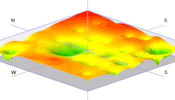
This program is used to generate a potentiometric surface model based on pumping and/or injection wells using the Theis non-equilibrium equation. Data for multiple wells is read from the main datasheet; varying saturated thickness measurements are allowed. The resulting surface can be displayed as a 2D map or 3D surface.
See also: Simplified drawdown (fixed thickness and transmissivity), and Anisotropic drawdown (separate X and Y transmissivity)
Menu Options
Step-by-Step Summary
Menu Options
- Input Columns: Use the prompts along the left side of the window to specify the names of the columns in the main datasheet that contain the necessary parameters:
- X (Easting): Click on this item to select the column in the datasheet that contains the X-coordinates for the wells.
Be sure you define your coordinate system and units for all columns except Storativity and Duraton.
- Y (Northing): Click on this item to select the column in the datasheet that contains the Y-coordinates for the wells.
- Pre-Pump Water Elevation: Click on this item to select the column that contains the well's pre-pump water elevation.
- Pumping Rate: Select the column in the datasheet that contains the pumping rates for the wells. Specify your units in gallons (Imperial units) or liters (metric units) per minute. Note: If the well is an injection well, the rate can be entered as a negative value.
- Well Radius: Select the column that contains the well radius measurements.
- Transmissivity: Click on this item to select the column that contains the transmissivity values. Required. Units are entered in gallons per day per foot (Imperial units) or square meters per day (metric units).
- Storativity: Choose the column that contains the storativity values.
- Saturated Thickness: Select the column in the datasheet that contains the saturated thickness measurements. Required: Units in feet or meters.
- Duration: Click here to select the column that contains the pumping duration. Required: Units in days. Note: Decimal days (e.g. 0.5 = 12 hours) are acceptable.
- Grid Name: Click to the right to type in the name to assign to the grid model (.RwGrd file) that the program will create, containing the model of the drawdown surface.
- Model Dimensions: Expand this item to establish the drawdown grid's dimensions. In general, the larger the number of grid cells (the "finer" the grid), the smoother the resulting map, but the slower the processing. Similarly, a smaller the number of grid cells will enhance the program’s speed but will produce a more discontinuous map.
- Create 2-Dimensional Grid Diagram: Insert a check here if you want to display the output grid as a 2D map at this time. Expand this heading to set up the 2D map layers (bitmap, symbols, labels, line contours, color-filled contours, labeled cells, and/or map border).
- To activate a layer, insert a mark in its check-box.
- To access the layer's settings, expand the item by clicking on its "+" button. Then either click on the available button or expand the additional tree menu headings.
- Create 3-Dimensional Grid Diagram: Insert a check here if you want to display the output grid as a 3D surface at this time. Expand this heading to set up the 3D options.
! You can request both a 2D and 3D representation of the grid model.
- 3D Surface Options: Click on this button to establish the color and other surface settings.
- Reference Cage: Check this box to include a 3D grid of reference lines and labels with the diagram. Expand this heading to access the cage options.
- Create Grid Statistics Report: Insert a check here if you want to see a report summarizing the output grid.
- Include Standard Deviation: Check this box if you want the report to include standard deviation.
- Include Directional Analysis: Check this box to include slope, aspect, and strike computations. Be warned that these can take a few moments for large grid models.
Step-by-Step Summary
- Access the RockWorks Utilities program tab.
- Enter/import your drawdown data into the datasheet. (Example: RockWorks17 Data\Samples\Drawdown_Isotropic_01.RwDat)
- Select the Hydrology | Drawdown Surface | Isotropic menu option.
- Enter the requested menu items, described above.
- Click the Process button to continue.
If you have activated the gridding Dimensions / Confirm Dimensions option, the program will display a summary window with the grid boundary coordinates and node spacing.
- Adjust the grid dimensions as necessary and click OK.
The program will computed the drawdown grid model, reading the source data from the current spreadsheet, and using the requested grid dimensions. The model will be saved on disk under the file name you specified.
If you have activated the Confirm Intervals setting for either Contour Lines or Color Intervals, the program will display a summary window with default contour intervals.
- Adjust these items if necessary and click OK. The z-value units in the map will represent feet of drawdown (if imperial units) or meters of drawdown (if metric units).
The program will read the completed drawdown grid model and, if requested, create a 2- or 3-dimensional image representing the grid model. The requested diagram(s) will be displayed in a RockPlot2D tab and/or RockPlot3D tab in the Options window. If you requested a statistics report, it will be displayed in a Text Tab in the Options window.
- View / save / manipulate / print / export the map in the RockPlot2D or RockPlot3D window.
 Back to Hydrology Menu Summary

RockWare home page