Tutorial: Create a Modeled P-Data Cross Section

Estimated time: 3 minutes.

In this lesson, you will create a multi-paneled set of section panels using the P-data model you created in the previous lesson. The instructions below are written with the assumption that you have completed the previous lesson, as well as the lesson on log sections.

1. Click on the P-Data menu and choose Section | Model-Based.
   
2. Main Options: These settings will set up the model and diagram settings. These are found in the left pane of the P-Data Section window.
   • Vertical Exaggeration: This should be set to 1.
   • 
     
   • Model: Establish the model settings.
     • Use Existing Model: Since you took the time to create a P-data solid model in the previous lesson, we can use that one for this tutorial.
     • Solid Model: Click here to browse for the file Gamma.RwMod.
       ! This is really important to remember ! In your own work. Once a solid, numerical model is created to represent your data, and saved as an ".RwMod" file, you can use that same model to create different types of diagrams – profiles, sections, fences, isosurfaces, slices – without having to recreate the solid model each time. Here we just want to create a new type of diagram from the model you already created.
     • 
       
   • Contour Options This tab includes settings that apply to both 2D and 3D grid displays:
   • • Color Bands – Click here to enable colored contour bands and specify a Color Scheme used for 2D Contour Maps or 3D Surface Diagrams.
     • Contour Lines – Click here to enable Contour Lines and specify settings for both 2D and 3D diagrams.
     • Smoothing – Click here to specify Contour Smoothing passes, which will be applied to both the Color Bands and Contour Lines. Note that contour smoothing is applied AFTER grid creation and is a separate step from the Grid Smoothing tools that can be applied during grid creation.

     • 

     • Labeled Cells – Click here to turn on Labeled Cells for 2D Grid Maps. The program will draw a grid of lines corresponding to the grid model nodes, and fill the cells with labels for the node values.
     • Gradient Vectors – Click here to turn on Gradient Vectors for 2D Grid Maps, The program will display small arrows between grid nodes to represent uphill or downhill gradients.
     • 
       
   • Striplogs: Checked. The program will append 2D logs to the section panels.
   • 
     
   • Annotation: Checked. The defaults from the earlier lesson should work.
   • 
     
   • or Plot Surface Profile: This option can be either checked or not, as per the log section lesson.
   • 
     
   • Infrastructure: Unchecked.
   • Other 2D Files: Unchecked.
   • Peripherals: Unchecked.
   • Border: Unchecked.
   • 
     
   • Output Options
     • Display: Checked.
     • Save: Unchecked.
     • Export: Unchecked.
     • 
       
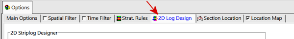
3. Check the striplog options: These should still be set up as they were for the log section; if you want to review the 2D log settings you can click on the 2D Log Design tab at the top of the window.
   

   

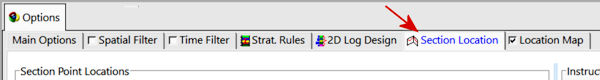
4. Check the selected boreholes: These should also still be set up as they were for the log section. To verify the placement of the section trace, click on the Section Location tab at the top of the window.

   

   

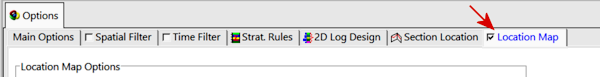
5. Location Map: This should still be checked as it was for the log section lesson. To verify the settings, click on the Location Map tab at the top of the window.

   

6. Faulting: Click on this tab to enable the display of faults and to modify fault options. (Read this for more details.)
   
7. Click the Continue button to accept the modeling and diagram options.

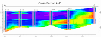
   • RockWorks will read the existing solid model (Gamma.RwMod) and extract panels along the indicated cross-section trace. It will build them into a continuous cross section diagram, with the indicated perimeter annotation. The curve logs will be appended to the section diagram. The completed diagram will be displayed in a RockPlot2D tab.

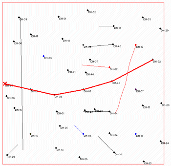
     The map representing the section panel trace will be displayed in a separate RockPlot2D tab.

   • You can save the section and map if you wish using the File | Save As menu command.
   • 
     
   • Close the window.
   
   

  P-Data Sections

  Back to P-Data menu     |     Next (fence diagram) 

RockWare home page