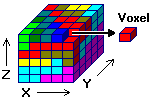

There are several methods offered to perform the 3-dimensional interpolation of your data. Each operates differently, and each has advantages and disadvantages. Click on a method below for more information.
Closest Point: Each solid model node is simply assigned the value of the closest control point. This can be used for real numbers as well as lithology modeling.
Directional: This method uses Inverse-Distance, allowing you to specify a trend direction and strength, and the program will vary the weighting exponent so that points along the trend influence the node more than closer points perpendicular to the trend.
Distance to Point: Each solid model node is assigned a value that represents its distance, in your X, Y, Z coordinate units, to the closest control point.
IDW Advanced (Inverse-Distance Weighting). This method uses the Inverse-Distance modeling algorithm, which uses a weighted average approach to compute node values. This particular method offers user control over the horizontal and vertical weighting of the control points, as well as all-point versus directional searching for the control points to use in modeling.
IDW Anisotropic (Inverse Distance Anisotropic): This uses Inverse-Distance, looking specifically at the closest point in each 90-degree zone around the node when assigning the node value. This method uses a fixed exponent.
IDW Isotropic (Inverse-Distance Isotropic): This also uses Inverse-Distance, using all control points and a fixed exponent when assigning node values.
IDW Layered (Inverse-Distance Isotropic): This also uses Inverse-Distance, using all control points within the specified layer height based on specified value when assigning node values.
IDW Table-Based (Inverse-Distance Table-Based): This method also uses Inverse-Distance, with specific search zones defined in a "Sector Table". You can also define the minimum number of points to be used from each sector and the exponent. Points that lie within the search sector(s) will be used in interpolation, and those that do not, will not.
Kriging - HB (Horizontally-biased Kriging): This method applies "2.5 D" Kriging to 3D data.
Lateral Blending: This method is used for lithology modeling and for modeling discrete (non-gradational) I-Data, T-Data, and P-Data values. This method extrudes the values horizontally from the boreholes (control points) outward, 1/3 of the way to the neighboring hole. In the middle zone it "feathers" the interpolation for less abrupt borders.
Lateral Extrusion: This method is also used for lithology modeling and for modeling discrete (non-gradational) I-Data, T-Data, and P-Data values. This method extrudes the values horizontally from the boreholes outward, to the midpoint between a neighboring hole.
Highest Probability: The Highest Probability algorithm starts by building a table of all unique g-values encountered within the control points. For each of these g-values, a probability model is created based on the inverse-square law (probability is inversely proportional to the square of the distance). The program then assigns the final node values based on the g-value with the highest probability.
Trilayer: This method is also used for representing layered but laterally discontinuous materials that do not laterally grade from one material type to another. The interpolation method creates a Delaunay triangle network for each layer and then projects the lithologies from the control points within that layer towards points that share the same triangle.
![]() Back to Creating Solid Methods
Back to Creating Solid Methods