
The Inverse-Distance Isotropic modeling method is one of the many "flavors" of the Inverse-Distance algorithm. Using Inverse-Distance in general, a voxel node value is assigned based on the weighted average of neighboring data points, and the value of each data point is weighted according the inverse of its distance from the voxel node, taken to a power (an exponent of "2" = Inverse-Distance squared, "3" = Inverse-Distance cubed, etc). The greater the value of the exponent, the less influence distant control points will have on the assignment of the voxel node value. For more information about Inverse-Distance algorithm, see Inverse-Distance Gridding.
Using the Inverse-Distance Isotropic method, the program will use all of the available data points when computing a voxel node’s value. The weighting exponent is set to "2" so that the data points are weighted according to the inverse of the square of their distance from the node.
Advantages: This is useful when modeling uniformly distributed data in non-stratiform environments.
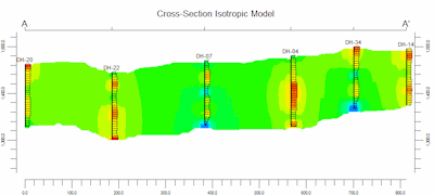
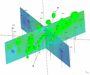
Disadvantages: If there are localized highs, this method can produce "bull's eyes" around the boreholes while the rest of the model is an average of the measured values.
There are no menu options to choose. Here are some examples of how isotropic models look in cross section and in 3D.
![]() Back to Solid Modeling Method Summary
Back to Solid Modeling Method Summary
![]()