
The Inverse-Distance Anisotropic modeling method is one of the "flavors" of the Inverse-Distance algorithm. Using Inverse-Distance in general, a voxel node value is assigned based on the weighted average of neighboring data points, and the value of each data point is weighted according the inverse of its distance from the voxel node, taken to a power (an exponent of "2" = Inverse-Distance squared, "3" = Inverse-Distance cubed, etc). The greater the value of the exponent, the less influence distant control points will have on the assignment of the voxel node value. For more information about Inverse-Distance algorithm, see Inverse-Distance Gridding.
Using the Inverse-Distance Anisotropic method, the program will look for the closest control point in each 90-degree sector around the node. For this method, the weighting exponent is also set to "2".
Advantages: This kind of directional search can improve the interpolation of voxel values that lie between data point clusters, and can be useful for modeling drill-hole based data in stratiform deposits. The quadrant searching tends to connect highs and lows at the same elevation.
Disadvantages: This option is slower than the Isotropic method since it has to filter neighboring points in assigning node values.
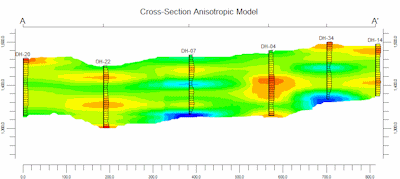
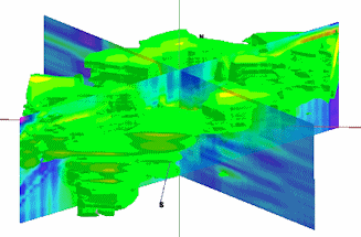
There are no menu options to choose. Here are some examples of how anisotropic models look in cross section and in 3D.
![]() Back to Solid Modeling Method Summary
Back to Solid Modeling Method Summary
![]()