The Inverse-Distance Weighting modeling method is one of the "flavors" of the Inverse-Distance algorithm. In general, when you use Inverse-Distance, a voxel node value is assigned based on the weighted average of neighboring data points, and the value of each data point is weighted according the inverse of its distance from the voxel node, taken to a power (an exponent of "2" = Inverse-Distance squared, "3" = Inverse-Distance cubed, etc). The greater the value of the exponent, the less influence distant control points will have on the assignment of the voxel node value. For more information about Inverse-Distance algorithm, see Inverse-Distance Gridding.
The Inverse-Distance Weighting method can use either all of the available data points when computing a node’s value or it can search for specific points. And, instead of automatically using a weighting exponent of "2", the program allows the user to assign different weighting exponents to control points oriented vertically versus horizontally from the node. The greater the exponent you enter, the less influence those data points will have.
Menu Options
- Weighting Exponents: This method allows you to vary the weighting exponent horizontally versus vertically. Because most data points will lie neither directly above, below, or horizontal to the node being interpolated, the program will adjust the exponent based on the inclination between the node and the control point.
- Horizontal: If you want to bias the modeling horizontally, you should set the Horizontal Exponent to a lesser value than the Vertical Exponent. For example, you could set the Horizontal Exponent to 2 and the Vertical Exponent to 5 to apply a horizontal bias to the modeling. Default = 2
- Vertical: If you want to bias the modeling vertically, you should set the Vertical Exponent to a lesser value than the Horizontal Exponent. Default = 2
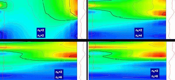
The examples below illustrates the effect of these exponents. Each image represents a slice of a geophysical solid model between two wells, with the geophysical curve shown on either side of the panel. Where both horizontal and vertical exponents = 2, there is little bias horizontally. Where the horizontal exponent = 2 and the vertical = 8, there is much greater horizontal bias.
- Search Method: Expand this heading to define how the program will locate the control points to use for modeling. These search options allow the user to minimize the effects of clustered data points (e.g. closely spaced points within widely separated drill holes).
- All Points: Choose this option if the modeling method is to use all control points when assigning node values. This is the faster option since there is no point searching and filtering to occur. This option works well when modeling groundwater plumes. (Note: If you've set the horizontal and vertical exponents to "2" and choose All Points, this is the same as Inverse-Distance Isotropic.)
- Fast Inverse Distance: For large datasets, this is a good option. It limits both the number of overall control points that will be used to interpolate a voxel value and the number of points per borehole to be used.
- Max Points per Voxel: Use this setting to define the maximum number of control points to be used to interpolate a voxel.
- Max Points per Borehole: This defines the maximum number of control points per borehole to be used for interpolation.
For example, if you defined the Max Points per Voxel to be 15 and the Max Points per Borehole to 5, the program will pull the 5 closest points in each of the three closest boreholes to interpolate each voxel.
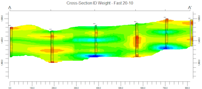
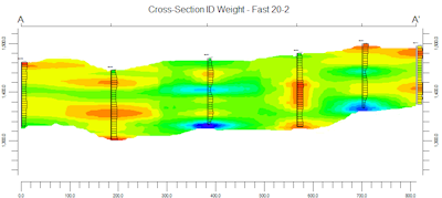
The fewer points per borehole, the more horizontal bias will be applied to the model. In the example on the left (below), the search method pulled 10 points per hole (20 points total). In the example on the right, the search method pulled 2 points per hole (20 total).
- Closest Points within Sector: Choose this option if you want to define specific sectors to search for control points.
- Sector Width: This defaults to 90 degrees, you can make the dividing angle smaller to increase the number of sectors from which control points will be pulled.
- Sector Height: This defaults to 90 degrees, you can make the dividing angle smaller to increase the number of sectors from which control points will be pulled.
(Note: If you've set the horizontal and vertical exponents to "2" and use 90-degree sectors, this is the same as Inverse-Distance Anisotropic.)
The following example depicts nine possible settings for the weighting exponents.
Note: You are not confined to integer settings for the weighting exponents. Zeroes are also ok. For example, the model on the left within the following diagram was based on horizontal and vertical exponents of 2.0. The model on the right is based on a horizontal exponent of zero and a vertical exponent of 6. Notice the pronounced lenticularity within the model on the right.
 Back to Solid Modeling Method Summary

RockWare home page