
RockWorks | Utilities | Grid | Directional Analyses |
Grid -> Downgradient Vector Map
This program reads a grid (surface) model and creates a 2D map containing small arrows at each grid node pointing downhill. Arrows may be scaled and/or color-coded according to steepness of slope.
Note: This program requires that a RockWorks surface (grid) model already exist.
Menu Options
Step-by-Step Summary
Menu Options
- Grid (Surface) Model: Click to browse for the name of the existing grid model (".RwGrd" file) to be analyzed and displayed as a vector map.
- Normalize Nodes Prior to Analysis: Leave this unchecked if your grid model represents topographic elevations.
If your grid model represents something other than topography (e.g. geochemical concentrations), you should check this box so that the Z values can be normalized to map units prior to computing the slope and aspect. For example, if a grid node spacing is 10 meters and the user is analyzing geochemical data than ranges between zero and 0.01, the maximum slope would be less than one degree in which case the program would produce a blank diagram. With normalization, however, the data is now rescaled to resemble a three-dimensional cube in which the slope will have a wide range (i.e. zero to 90 degrees).
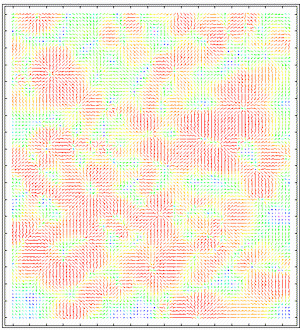
- Automatic: Using this normalization scheme, the program will rescale the grid node values such that the minimum node value will represent zero while the maximum node value will be equal to the map distance from the southwest corner to the northeast corner of the grid model. The map below illustrates a downgradient vector map based on normalized geochemical data that initially ranged between zero and 0.01.
- Manual: Choose this option if you want to enter your own min and max range within which the grid node values are to be normalized before the analysis is run.
- Minimum/Maximum Dip: Enter the minimum and maximum slope values to be included in the map. Enter "0" for the minimum and "90" for the maximum if all nodes are to be included. Or, to show only those nodes with slope > 30 degrees, for example, you would enter "30" for the minimum and "90" for the maximum.
- Arrow Length:
- Choose Fixed if you want the map arrows to be the same length, roughly the same size as the node-to-node spacing.
- Or, choose Proportional if you want each map arrow's length to be scaled based on its slope, with flat areas plotting with short arrows and steep arrows with long arrows.
- Arrow Colors:
- Choose Fixed to set the arrows to a single color, and expand the Fixed item to select the color.
- Or, choose Variable to set the arrows to a variable scheme, using cold colors for nodes with shallow slopes and hot colors for nodes with steep slopes, and graduating the colors in-between.
- Arrow Thickness: Click here to select the line thickness for the arrows. "1" will generate thin lines, "3" thick ones.
Step-by-Step Summary
- Be sure you have a RockWorks grid model already created, for input into this program.
- Access the RockWorks Utilities program tab so that you can see the Grid menu. It is not necessary to open a datasheet.
- Select the Grid | Directional Analyses | Grid -> Downgradient Vector Map menu option.
- Enter the requested menu settings, described above.
- Click the Process button to continue.
The program will read the input grid model, compute slope and aspect for each node, and then create a map that indicates the down-slope gradient with arrows, using the requested map settings. The map will be displayed in a RockPlot2D tab in the Options window.
- You can adjust any of the settings in the Options window (arrow settings, grid model name, etc.) and then click the Process button again to regenerate the map.
! Each time you click the Process button, the existing display will be replaced.
- View / save / manipulate / export / print the map in the RockPlot2D window.
Tip: Use RockPlot2D's File | Export | RockPlot3D option to drape this downhill gradient map over the original grid surface for display in RockPlot3D.
 Back to Grid Menu Summary

RockWare home page